Arrowheads

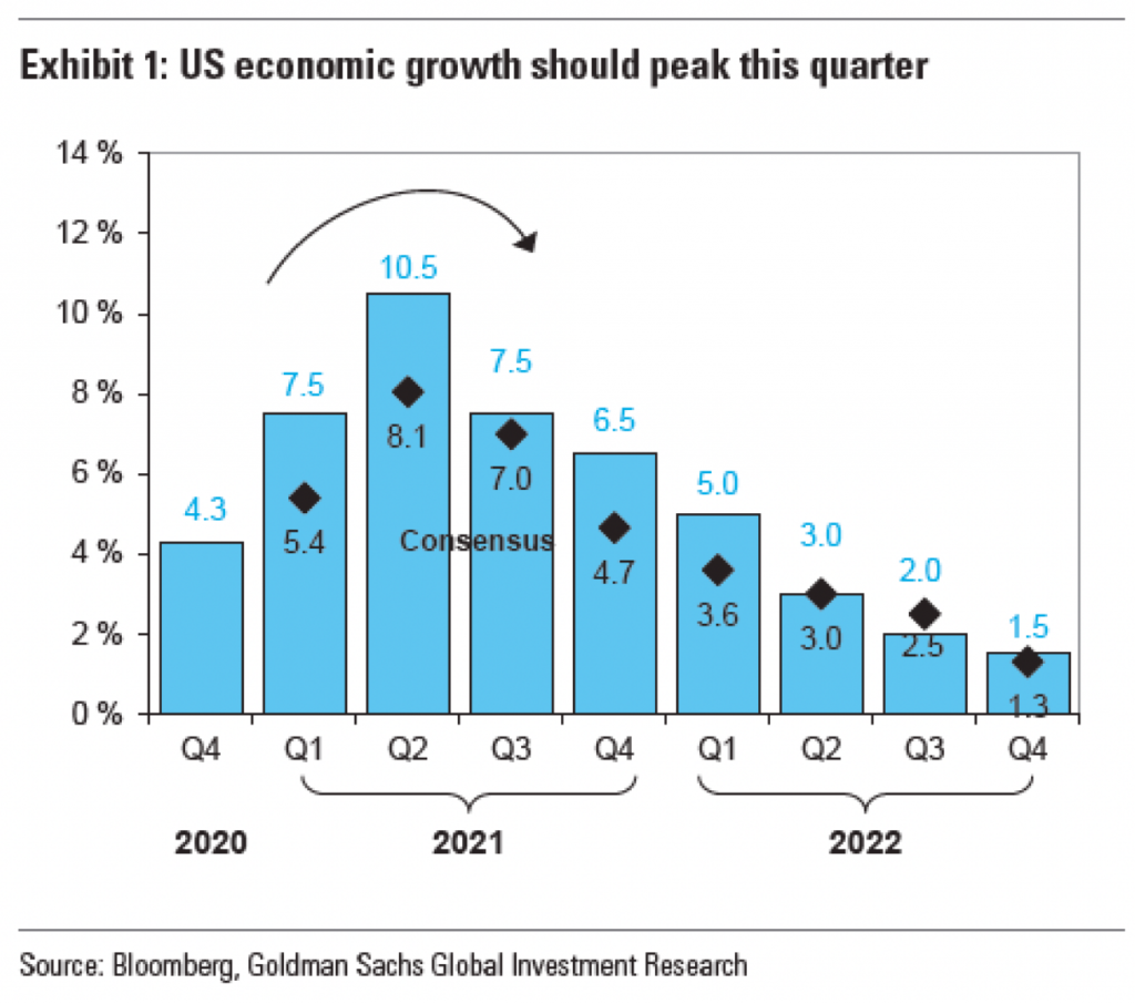
I don’t know if this is a trend, but I’ve now seen a few graphics appearing using arrows to show the direction or trend of the data. This graphic in an article by Bloomberg prompted me to talk about this piece.

I should add, after rereading my draft, that I’m not clear who made this graphic. I assume that it was the Bloomberg graphics team, because it appears in Bloomberg and all the data is presented to recreate the chart. But, it could also be a chart made by someone at Goldman Sachs that credits Bloomberg as a source and then someone at Bloomberg got hold of a copy. And a graphic made for a news/media outlet will typically be of a different quality or level of polish than one made perhaps by and for analysts. (Not that I think there should be said differences, as it does a disservice to internal users, but I digress from a digression.)

All the things going on in this chart.

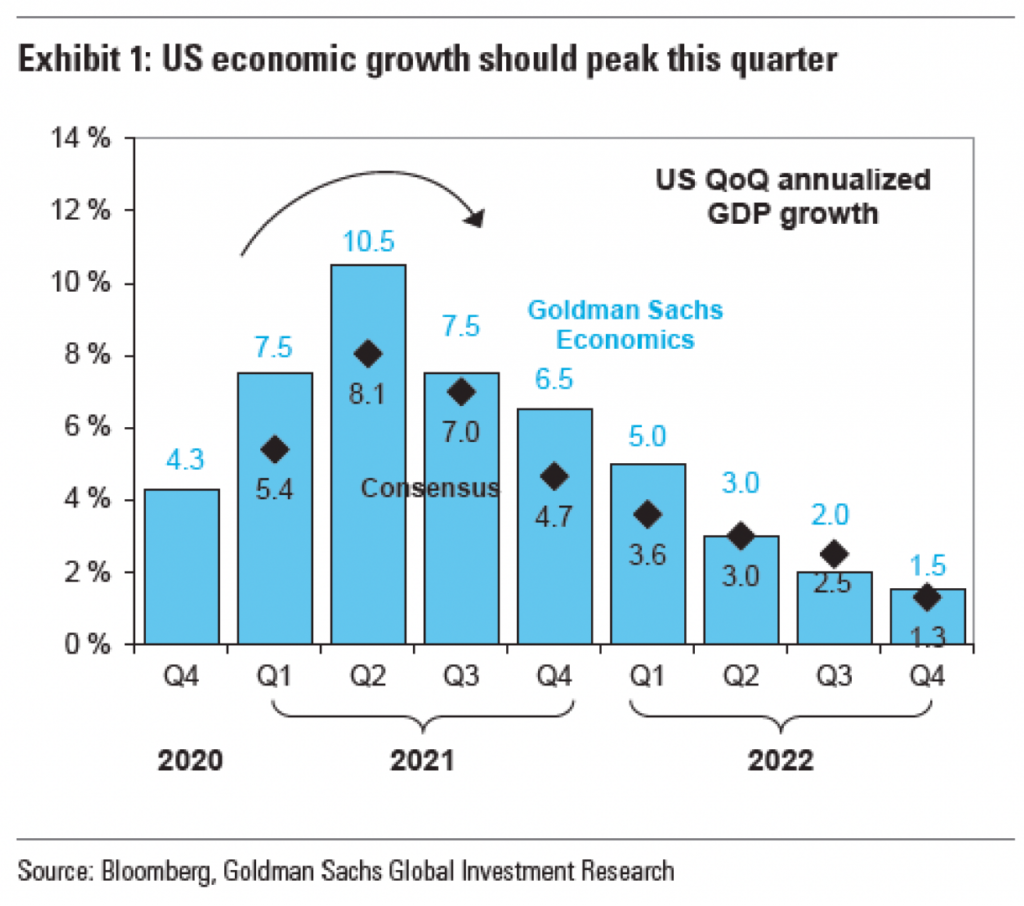
The arrow here appears above the peak quarter, i.e. the second of 2021, for both the Goldman Sachs Economics forecast and the consensus forecast. But what does it really add? First, it adds “ink”, in this case pixels. Here, every pixel consumes our attention and there is a finite number of available pixels within the space of this graphic.

When I work with authors or subject matter experts, I often find myself asking them “what’s the most important thing to communicate?” or something along those lines. If the person answers with a long laundry list, I remind them that if everything is important, nothing is important. If everything is set in bold, all caps text, what will look most important is the rare bit of text set in regular, lower-case letters.

In the above graphic, there are so many things screaming for my attention, it’s difficult to say which is the most important. First, I’m fairly certain that “US QoQ annualised GDP growth” could move to the graphic subhead or data definition. Allow the graphic’s data container to contain, well, data. Second, the data series labels can be moved outside the data container. The labels here have an inherent problem is that the Goldman Sachs Economics numbers are in blue, and that blue text has less visual weight than the black text of the Consensus label. Consequently, the Goldman Sachs Economics label recedes into the background and becomes lost, not what you want from your legend.

Third, I don’t believe the data labels here add anything to the chart. They function as sparkly distractions from the visual trend, which should be the most important aspect of a visual chart.

Finally, we get to the arrow, the impetus for this post. First, I should note that it is not clear what growth it shows. The fact the line is black makes me think it reflects the Consensus forecast whereas a blue line would represent the Goldman Sachs forecast. But it could also be the average of the two or even a more general “here’s the general shape”. The problem is that the shape matters. If you look at the slope of the actual forecasts, you see a sharp increase to the peak followed by a slower, more gradual taper. The arrow in the original graphic shows a decelerating curve that is shallower in the lead up to the peak and that is not what is forecast to happen.

Now we get to the issue I mentioned at the top, the extraneous labelling and data ink wasted. If we look at the chart as is, but remove the arrow, we see this.

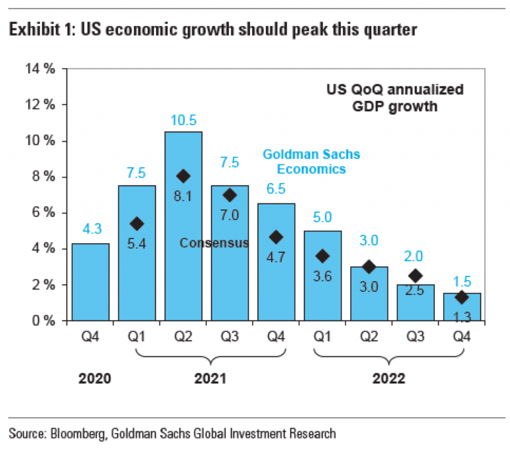
Immediately to the right of the peak, we have have some blue data labels and then just a bit to the right of that, but sitting vertically above the label we have the bold blue text labelling the data series. But further to the upper right we have a dark and bold block of text that draws the eye away from the peak and into the corner. It draws the eye away from the very element of the shape the peak needs to be a peak, the trough in the wave. Consequently, it makes sense with the eye being drawn up and to the right that the designers threw an arrow in above the peak to show how, no, actually your eye needs to go down and to the right.

But what happens if we then strip out the data series labelling? Do we still need the arrow? Let’s take a look.

I would argue that no, we do not. And so let’s strip the arrow out of the picture and take a look.

Here the shape of the curve is clear, a sharp rise and then a gradual taper to the right. No arrow needed to show the contour. In other words, the additional labelling wastes our attention, which then forces us to add an arrow to see what we needed to see in the first place, but then further wasting our attention.

There are a number of other things I take issue with in this chart: the black outlines of the blue rectangles, the tick marks on the x-axis, the solid border of the container, the lack of axis lines. But the arrow points to this graphic’s central problem, a poorly thought out labelling structure.

So because the chart provides all the data, I took a quick stab at how I would chart it using my own styles. I gave myself a 3:2 ratio, less space than the original graphic had. This is where I landed. I would prefer the legend below the chart labelling, but it felt cramped in the space. And with so few data points along the x-axis, the chart doesn’t need a ton of horizontal space and so I repurposed some of it to create a vertical legend space.

I mixed typefaces only because my default does not have a proper small capitals and I wanted to use small capitals to reduce and balance out the weight of the exhibit label in the graphic title.

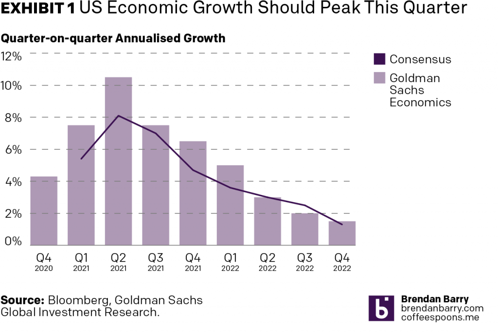
I could still tweak the spacing between the bars and perhaps the treatment of the years below the quarters could use some additional work, but the main point here is that the shape of the curve is clear. I need no arrow to tell the user that there is a peak and that after the peak the line goes down. The white space around the bars and the line does that for me.

Credit for the piece goes to either the Bloomberg graphics department or the Goldman Sachs graphics department. Not sure.

What Will the Next Recovery Look Like?

Earlier this morning, the Bureau of Economic Analysis released its US 2nd quarter GDP figures and the news…isn’t great. On an annualised basis, we saw -32.9% growth. That’s pretty bad. Like Great Depression level bad. I’ve posted on the social media how bad this current recession is and how nobody in the workforce today worked or didn’t through the Great Depression to really relate to the numbers we are seeing.

But that’s all today. The sun will come out tomorrow. (And scorch the Earth as climate change renders certain parts of the globe uninhabitable to mankind. But we’ll get to those posts in later weeks.) And when it does come out, eventually, what will the recovery look like? I’ve seen a few mentions recently in the media of a V-shaped recovery. What is this mysterious V-shape?

A long time ago, in a galaxy far away. Or during the last recession in Chicago, I worked with some really smart people in some of my professional projects and we covered the exact same question. There are a couple key “shapes” to an economic recovery. And when we say recovery, we mean just to return to pre-recession peak levels of growth. Anything above that is an expansion. That’s what we want to get back to.

What kind of shape will the recovery take?
Who knew typographers loved economics?

The V-shape we hear a lot about is a sharp recovery after the economy bottoms out (the trough). Broadly speaking, if a recession has to last two consecutive quarters (it doesn’t, but that’s a pretty common definition so let’s stick with it), then in a V-shape, we are talking about a recovery one or two quarters later.

Similar to the V is the W-shape, where things start to improve rapidly, but some kind of shock to the economic system and things go back negative once again before finally picking up quickly. It’s not hard to imagine something going horribly wrong with the Covid-19 pandemic to be just that external shock that could push the economy back down again.

Similar still is the U-shape. Here, after hitting rock bottom, growth isn’t quite as quick to pick up as we linger in the depths of the valley of recession. But after a bit of time, we again see a rapid recovery to pre-recession levels of growth.

These are all pretty short term recoveries, the W being a little bit longer because two sharp downturns. But they are nothing compared to what’s also possible.

First we have the L-shape. Here, after hitting bottom, things start to recover quickly. But that recovery is slow and takes a long time. Growth remains slower than average, creeping up to average, and then still takes its time to reach pre-recession levels. Is something like this possible? Well, if vaccines fail and if some countries still can’t get their act together (cough, US, cough), the willingness of consumers to go out, eat, drink, buy things, travel, and generally make merry could be suppressed for a long time. So it’s certainly not out of the question.

And then lastly we have the UUUU-shape. Though you could probably add or subtract a U or two. This features more drawn out stays at the bottom of the valley with quick and sharp upticks in growth. But those growths, never reaching pre-recession levels, also collapse quickly back into declines, though also never really reaching the same depths as earlier. Essentially, the recovery faces multiple setbacks knocking the economy back down as it sputters to life. As with the L-shape, it’s also not hard to imagine a world where a country hasn’t managed to contain its outbreak struggling to get back on its feet.

What do you think? Are we at rock bottom? Did I miss a recovery type?

Credit for the graphic is mine.

Trump-won Counties Are Winning

Yesterday we looked at how China and the European Union are planning their tariff/trade war retaliation to target Trump voters. Today let’s take a look at how those voters are doing as this article from Bloom does.

Lots of green, but some noticeably red counties in Florida.

The article is not terribly complicated. We have four choropleth maps at the county level. Two of the maps isolate Trump-won counties and the other two are Clinton-won. For each candidate we have a GDP growth and an employment growth map.

In the Trump-won maps, the Clinton-won counties are white, and vice versa. Naturally, because the Democratic vote is greatest in the large cities, which, especially on the East Coast, are in tiny counties, you see a lot less colour in the Clinton maps.

Not a whole lot to see here…

Design wise, I should point out the obvious that green-to-red maps are not usually ideal. But the designers did a nice job of tweaking these specific colours so that when tested, these burnt oranges and green-blues do provide contrast.

Here they appear more of a yellow to grey

But I am really curious to see this data plotted out in a scatter plot. Of course the big counties in the desert southwest are noticeable. But what about Philadelphia County? Cook County? Kings County? A scatter plot would make them equally tiny dots. Well, hopefully not tiny. But then when you compare GDP growth and employment growth and benchmark them against the US average, we might see some interesting patterns emerge that are otherwise masked behind the hugeness of western counties.

But lastly. And always. Where. Are .Alaska. And. Hawaii? (Of course the hugeness problem is of a different scale in Hawaii. Their county equivalents are larger than states combined.)

Credit for the piece goes to the Bloomberg graphics department.

The World Grows On (Part III)

A few days ago I posted about the front cover graphic for the New York Times that used a choropleth to explore 2017 economic growth. Well, this morning whilst looking for something else, I came across the online version of the story. And I thought it would be neat to compare the two.

A very nice graphic
A very nice graphic

Again, nothing too crazy going on here. But the most immediately obvious change is the colour palette. Instead of using that green set, here we get a deep, rich blue that fades to light very nicely. More importantly, that light tan or beige colour contrasts far better against the blue than the green in the print version.

The other big change is to the small multiple set at the bottom. Here they have the space to run all twelve datasets horizontally. In the earlier piece, they were stacked six by two. It worked really well, but this works better. Here it is far easier to compare the height of each bar to the height of bars for other countries.

Credit for the piece goes to Karl Russell.

The World Grows On

January is the month of forecasts and projections for the year to come. And the Economist is no different. Late last week it published a datagraphic showcasing the GDP growth forecasts of the Economist Intelligence Unit. I used to make this exact type of datagraphic a lot. And I mean a lot. But what I really enjoy is how successfully this piece integrates the map, the bar chart, and the tables to round out the story.

Take a note at how the chart distributes the bins as well

The easy thing to do is always the map, because people like maps. They can be big, and if the data set is robust, full of data and colour. But maps hide and obscure geographically small countries. And then you have to assume that people know all the countries in the world. Problem is, most people do not.

So the bar chart does a good job of showing each country as equals, a slim vertical bar. In such a small space, labelling every country is impossible, but the designers chose a select number of countries that might be of interest and called them out across the entire series.

Lastly, people always like to know who is #winning and who is a #loser. So the tables at the extreme ends of the chart showcast the top and last five.

I may have rearranged some of the elements, and dropped the heavy black rules between the bins on the legend, but overall I consider this piece a success.

Credit for the piece goes to the Economist Data Team.

Declining British Wages

Now for the actual piece for today.

We have a scatterplot from the Financial Times that looks at wage and economic growth across the OECD, focusing on the exception that is the United Kingdom. And that is not an exception in the good sense.

The UK had the rare privilege of experiencing economic growth—that’s good—while simultaneously wages fell—that’s bad. But I wanted to comment on the chart today.

I would have designed this a little bit differently

Straight off the bat, the salmon-coloured background does not bother me. That is FT’s brand and best to stick to it and make your graphics work around it. Possibly the colours in the plot could use a bit of a push to increase separation, but that is more a design quibble. Instead, I am not too keen on the colour coding here.

Not that the colours need not be applied, but why to the dots? Note how the dots of a colour fall into one of the quadrants. Instead of having people refer to the legend, incorporate the legend into the chart by moving the labels to the plot background. You could colour code the labelling or even colour the quadrants to make it a bit clearer.

Credit for the piece goes to the Financial Times graphics department.