Facebook’s for the Old Folks

We start this work week with something that the young people use, but in a different way than older people do, including elder millennials like myself: social media. Of course, as an elder millennial, I remember Facebook when it was The Facebook when it expanded access to Penn State, which I attended for a single year.

Pew Research conducted a study of teenagers that revealed they use social media more than ever before, but that they use new (sort of) platforms more than the venerable paragon of the past: Facebook.

The Economist’s Data Team looked at the data and created this graphic showing the trends.

What do you use? How often?

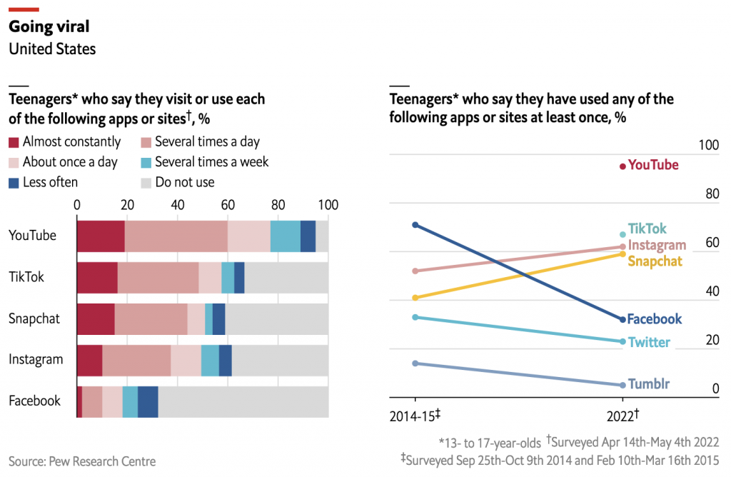
We see stacked bar charts on the left and then a line chart on the right. The left-hand chart shows the frequency with which teenagers use various social media platforms. What I don’t understand is how someone uses a social media application “almost constantly”. But that’s probably why I’m an elder millennial.

Get off my lawn, you whippersnappers.

On the right we see the percentage of teenagers who have used an application at least once. The biggest winners? Applications primarily featuring image over text. The losers? Those that use words.

Now longtime readers know that I am not terribly fond of stacked bar charts, especially because they make comparisons between, in this case, social media platforms very difficult. And I feel like we have a story in the occasional use responses, but it’s tough teasing it out from this graphic.

On the right, well, this is one I enjoy. You can tell just how much the social media environment has evolved in the last 7–8 years because TikTok did not exist and YouTube was not thought of as a social media platform.

I wonder if different colours were truly needed for the line chart. The lines do not really overlap and there is sufficient separation that each line can be read cleanly. If the designers wanted to highlight the fall of Facebook or another story line, they could have used accent colours.

But overall a solid graphic.

Now to check my feeds.

Credit for the piece goes to the Economist’s Data Team.

May Jobs Report

Friday the Bureau of Labour Statistics published the data on the jobs facet of the American economy. Saturday morning I woke up and found the latest New York Times visualisation of said jobs report waiting for me at my door. The graphic sat\s above the fold and visually led the morning paper.

Almost out of the hole.

We have a fairly simple piece here, in a good way. Two sections comprise the graphic. The first uses a stacked bar chart to detail the months wherein the US economy lost jobs during the previous two and a half years. We can take a closer look in this second photo that I took.

But the recovery hasn’t been uniformly good for all.

Here we can see the stacked bars pile up with the most recent bars to the right. Some of the larger bars have labels stating the number of jobs either lost (top) or gained (bottom). I’m not normally a fan of stacked bar charts, because they don’t allow a reader to easily discern like-for-like changes. In this instance, the goal is to show how close all the little bits have come towards making up the three negative bars. Where I take issue is that I would prefer the designers used some sort of scale to indicate even a rough sense of how many jobs the various bars represent.

That issue crops up again to a slightly lesser degree with the bottom set of graphics. These compare the growth of hourly earnings and inflation both from February 2020. During the first few months of the pandemic and its recession, you can see earnings for those most directly impacted by shutdowns drop. But there is no negative scale accompanying the positive scale and that makes it difficult to determine just how far earnings fell for those in, say, leisure and hospitality.

The second part of the graphic works overall, however it’s just some of the finer design details that are missing and take away from the graphic’s overall effectiveness.

This all fits part of a larger trend in data visualisation that I’ve been noticing the last few months. Fewer charts seem to be using axes and scales. It’s not a good thing for the field. Maybe some other day I’ll write some things about it.

For this piece, though, we have an overall solid effort. Some different design decisions could have made the piece clearer and more effective, but it still does the job.

Credit for the piece goes to Ben Casselman, Ella Koeze, and Bill Marsh.

School Shootings

The Wall Street Journal put together a nice piece about the uptick in elementary school shootings, both in the number of shootings and the number of deaths. It used two bar charts, regular and stacked, and a heat map to tell the story. The screenshot below is from a graphic that looks at the proportion of school shootings that occur at elementary schools. They are not as common, but as other graphics in the article show, they can be quite deadly.

Not a great trend…

The graphic above does a nice job of distilling the horror of a tragedy into a single rectangle. That is an important task because it allows us to detach ourselves and more rationally analyse the situation. Unfortunately the analysis is that yes, Virginia, things really have been getting worse.

Overall the article is simple but soberingly effective. School shootings are a problem with which American society has not dealt and my cynical side believes with which we will continue to not deal.

Credit for the piece goes to James Benedict and Danny Dougherty.

Substandard Housing in Philadelphia

I took a holiday yesterday and headed down the street to the Philadelphia City Archives, which houses some of the oldest documents dating back to the founding of the colony. But I was there primarily to try and find deeds and property information for my ancestors as part of my genealogy work.

When I walked into the building—the archives moved a few years ago from an older building in University City into this new facility—an interactive exhibit confronted me immediately. Now I did not take the time to really investigate the exhibit, because I anticipated spending the entire day there and wanted to maximise my time.

But there was this one graphic that felt appropriate to share here on Coffeespoons.

Philadelphia’s population crested in the 1950 census, it would decline continually until the 2010 census.

Like a lot of statistical graphics from the mid-20th century we have a single-colour piece because colour printing costs money. It makes use of a stacked bar chart to highlight the share of housing in the city that can be classified as substandard, i.e. dilapidated or without access to a private bath.

The designer chose to separate the nonwhite from the white population on different sides of the date labels, though the scale remains the same. I wonder what would have happened if the nonwhite bars sat immediately below the white bars within each year. That would allow for a more direct comparison of the absolute numbers of housing units.

That would then free up space for a smaller chart dedicated to a comparison of the percentages that are otherwise written as small labels. Because both the absolutes and percentages are important parts of the story here.

The white housing stock increased and the number of substandard units decreased in an absolute sense, leading to a strong decline in percentages.

But with nonwhite housing, the number of substandard units slightly increased, but with larger growth in the sheer number of nonwhite housing units overall, that shrank the overall percentage.

Put it all together and you have significant improvements in white housing, though in an absolute sense there still remain more substandard units for whites than nonwhites. Conversely, we don’t see the same improvements in housing for nonwhites. Rather the improvement from 45% to 35% is due more from the increase in housing units overall. You could therefore argue that nonwhite housing did not improve nearly as much as white housing between 1940 and 1950. Though we need to underline that and say there was indeed improvement.

Anyway, I then went inside and spent several hours looking through deed abstracts. Not sure if those will make it into a post here, but I did have an idea for one over a pint at lunch afterwards.

Credit for the datagraphic goes to some graphics person for some government department.

Credit for the exhibit goes to Talia Greene.

What Is Infrastructure?

This morning I read a piece in Politico Playbook that broke down President Biden’s $2.25 trillion proposal for infrastructure spending. A thing generally regarded as the United States sorely needs. $2.25 trillion is a lot of money and it’s a fair question to ask whether all that money is really money for infrastructure.

Because, it turns out, it’s not.

Please, sir, may I have more train money?

That isn’t to say money spent on job retraining or home care services wouldn’t be money well spent. Rather, it’s just not infrastructure.

But politics and the English language is a topic for another day. Oh wait, somebody already did write about that.

Credit for the piece is mine.

Biden’s Cabinet

Note: I wanted this to go up on Inauguration Day, but I had some server issues last week. And while I got everything back for Friday and Monday, I didn’t want to wait too long to post this. You’ll note at the end that I have questions about General Austin and whether he could be confirmed as Defence Secretary. Spoiler: He was.

Today is Inauguration Day and at noon, President Trump returns to being a citizen and Joe Biden assumes the office of the presidency. He comes to office with arguably the most diverse cabinet in American history supporting him and his agenda.

CNN took a look at that diversity with this piece, which uses an interactive, animated stacked bar chart.

The proposed cabinet vs. the US ethnic breakdown

I took a screenshot at the ethnic/racial diversity. At the top, each bar represents one member of cabinet who you can reveal after mousing over the bar. Below is a stacked bar chart showing the racial makeup of the United States. You can see how it does resemble, and in some cases exceeds, the diversity of the broader United States.

One thing to note, however, is that we see 26 members of Cabinet. Some of those are the heads of the big executive departments like Treasury and Defence. But I’m not certain everyone is technically a cabinet-level position, e.g. Celia Rouse, Chair of the Council of Economic Advisors. It could be that the position is being elevated to cabinet level like John Kerry’s role as climate envoy. And if I just missed the press announcement, that’s on me. But that could affect the overall numbers.

Regardless, the nominated cabinet is more diverse than the previous two administrations as the CNN piece also shows.

The proposed cabinet vs. the preceding inaugural cabinets

I should point out that usually an incoming administration usually has a few of its national security positions already confirmed or confirmed on the first day, e.g. Defence and State. However, the Republican Senate, obsessed with the lie of a fraudulent election, has only just begun to start the confirmation process. In fact, as of late last night, only Avril Haines has been confirmed by the Senate (84–10) for Director of National Intelligence.

Furthermore, almost every administration has one or two nominations that fail to pass the Senate. George W Bush had Linda Chavez, Barack Obama had Tom Daschle, and Donald Trump had Andrew Puzder, just to give one from each of the last three administrations.

With a 50–50 Senate, I would expect there to be a few nominees who fail to make it over the line. Austin could be one, there appears to be some bipartisan agreement that we ought not nominate recent military officials as civilian heads of said military. Another to keep an eye out for is Neera Tanden. She riles conservatives and angers Bernie Sanders supporters, so whether the Senate will confirm her as Director of the Office of Management and Budget remains an open question in my mind.

Credit for the piece goes to Priya Krishnakumar, Catherine E. Shoichet, Janie Boschma and Kenneth Uzquiano.

Can Texas Go Blue on Tuesday?

One story I’m following on Tuesday night is Texas. The state’s early voting—still with Monday to go—has surpassed the state’s total 2016 vote. Polling suggests that early votes lean Biden due to President Trump’s insistence that his supporters vote in person on Election Day as he lies about the integrity of early and mail-in voting.

The Texas Tribune looked at what we know about that turnout and what it may portend for Tuesday’s results. And, to be honest, we don’t—and won’t—really know until the votes are counted. They put together a great piece that divided Texas counties into four groups (their terminology): big blue cities, fast-changing counties, solidly red territory, and border counties. They then looked at the growth in registered voters in those counties from 2016, and looked at how they voted in the 2016 presidential election (Hillary Clinton vs. Donald Trump) and the 2018 US Senate election (Beto O’Rourke vs. Ted Cruz).

The piece uses the above stacked bar chart to show that Texas’ 1.8 million new registered voters’ largest share belongs to the big blue cities. The second largest group is the competitive suburbs in the fast-changing counties. The third largest, though quite close to second, was the solidly red territory. The border counties, still important for the margins, ranks a distant fourth.

I’m not normally a fan of stacked bar charts, because they do not allow for great comparisons of the constituent elements. For example, try comparing any of of those solidly red territory counties to one another. But here, the value is more in the stacked set as a group rather than the decomposition of the set, because you can see how the big blue cities have, as a group, a greater number of those 1.8 million new voters.

Those fast-changing counties include a lot of the suburbs for Texas’ largest cities. And those are areas where, across the country, Republicans are losing voters by the tens of thousands to the Democrats. As battlegrounds, these presented a challenge, because as swing counties, they split their votes between Clinton and Cruz and Trump and Beto. And so the designers chose purple to represent them in the stacked design. I think it’s a solid choice and works really well here.

But in terms of the story, I’ll add that in 2016, Trump won Texas by 807,000 votes. Texas added 1,800,000 new voters since then. And turnout before Election Day is already greater than it was in 2016.

It’s still a state likely to go for Trump on Tuesday. But, if Biden has a good night, it’s not inconceivable that Texas flips. FiveThirtyEight’s polling average has Trump with only a 1.2 point lead.

Credit for the piece goes to Mandi Cai, Darla Cameron and Anna Novak.

Which of These Countries Does Not Belong

For those of you reading from the States, I hope you all enjoyed your holiday. And for my UK readers, I hope you all enjoyed your summer bank holiday last weekend. So now to the good and uplifting kind of news.

Something is clearly not right here.

Indeed, a chart about deaths from firearms from the Economist. From a graphical standpoint, we all know how much I loathe stacked bar charts and this shows why. It is difficult for the user to isolate and compare the profiles of certain types of firearm violence against each other. Clearly there are countries where suicide by gun is more prevalent than murder, but most on this list are more murder happy.

And then the line chart that is cleverly spaced within the overall graphic, well, it falls apart. There are too many lines highlighted. Instead, I would have separated these out into a separate chart, made larger, so that the reader can more easily discern which series belongs to which country. Or I would have gone with a set of small multiples isolating those nine countries.

I am also unclear on why certain countries were highlighted in the line chart. Did they all need to be highlighted? Why, for example, is Trinidad & Tobago. It is not mentioned in the article, nor is it in the stacked bar chart.

But the biggest problem I have is with the data itself. But, every one of the countries on that list is among the developing countries or the least developed countries. Except one. And that, of course, is the United States.

Credit for the piece goes to the Economist Data Team.

The Economic Impact of Hurricanes

Yesterday Hurricane Ophelia hit Ireland and the United Kingdom. Yes, the two islands get hit with ferocious storms from time to time, but rarely do they enjoy the hurricanes like we do on the eastern seaboards of Canada, Mexico, and the United States.

Earlier this hurricane season the US had to deal with Harvey, Irma, and Maria. And in early October the Wall Street Journal published a piece that looked at the economic impact of the former two hurricanes as exhibited in economic data.

Overall the piece does a nice job explaining how hurricanes impact different sectors of the economy, well, differently. And wouldn’t you know it that leisure and hospitality is the hardest hit? But then they put together this stacked bar chart showing the impact of the hurricanes on both Florida/Georgia and Texas for Irma and Harvey, respectively.

I just want a common baseline…

The problem is that the stacked bar chart does not allow us to examine each hurricane as a specific data set. Because the Harvey data set is first, we have the common baseline and can compare the lengths of the magenta-ish bars. But what about the blue sets for Irma? How large is natural resources and mining compared to professional and business services? It is incredibly difficult to tell because neither bar starts at the same point. You must mentally move the bars to the same baseline and then hope your brain can accurately capture the length.

Instead, a split bar chart with each sector having two bars would have been preferable. Or, barring that, two plots under the same title. Then you could even sort the data sets and make it even easier to see which sectors were more important in the impacted areas.

Stacked bar charts work when you are trying to show total magnitude and the breakdowns are incidental to the point. But as soon as the comparison of the breakdowns becomes important, it’s time to make another chart.

Credit for the piece goes to Andrew Van Dam.

O’Reilly’s Out

Of all the things I expected to cover this week, this was not one of them.

This is Fox New’s firing of Bill O’Reilly, their lead personality and heaviest hitter for the last 21 years, for accusations of sexual harassment both externally and internally. But up until yesterday afternoon, just how important was O’Reilly to Fox News? Well, as you might guess somebody covered just that question. The New York Times addressed the question in this online piece and uses a nice graphic to buttress their argument.

What goes up must eventually fall down

I like the use of the longer time horizon across the top of the graphic. But most important in it is the inclusion of the trend line. It helps the reader find the story amid the noise in the weekly numbers. The big decline towards the end of December looks important until one realises that it probably owes the drop to the Christmas holidays.

Then the bottom piece does something intriguing; it shows both the actuals and percentages side-by-side. Typically people love stacked bar charts—by this point you probably all know my personal reluctance to use them—and that would be that. But here the designer also opts to show the share as a separate data point beside the stacked bar charts.

I think the only thing missing from the piece is a bit more context. Is O’Reilly still the heaviest weight in the lineup? The top chart could have perhaps used some additional context of other shows over the last few months. For example, how does O’Reilly compare to Hannity?

Regardless, this piece does a fantastic job of showing the until-yesterday increasing importance of O’Reilly to Fox News and then Fox News’ importance to 21st Century Fox.

Credit for the piece goes to Karl Russell.