Last week the Guardian published an article about drinking water pollution across the United States. Overall, it was a nicely done piece and the graphics within segmented the longer text into discrete sections. Each unit looks similar:
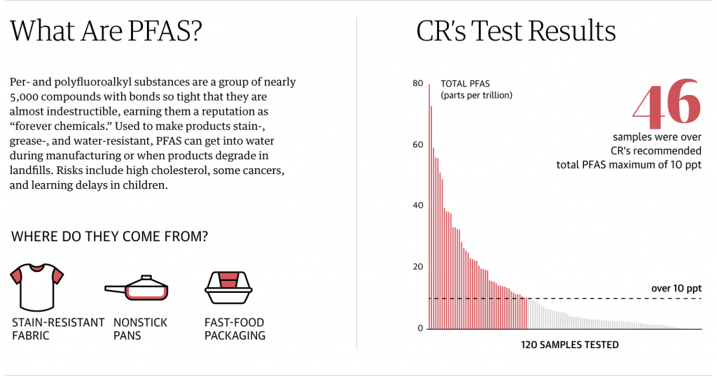
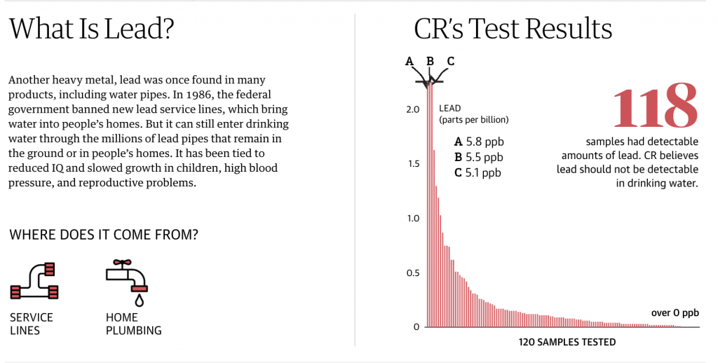
The left focuses on a definition and provides contextual information. It includes small illustrations of the mechanisms by which the pollutant enters the water system. To the right is a chart showing the levels of the contamination detected in the 120 tests the Guardian (and its partner Consumer Reports) conducted.
In almost all of the charts, we see the maximum depicted on the y-axis. And the bars are coloured if that observation station exceeds the health and safety limits. (The limit is represented by the dotted line.)
But towards the end of the piece we get to lead, a particularly problematic pollutant. There is no safe level of lead contamination. But how the piece handles the lead chart leaves a bit to be desired.
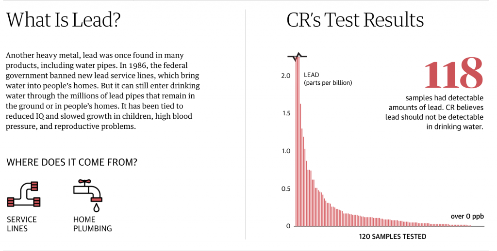
The first thing is colour, but that’s okay. Everything is red, but again, there is no safe level of lead so everything is over the limit. But look at the y-axis. That little black line at the top indicates a discontinuity in the lines, in other words the values for those three observations are literally off the chart.
But does that work?
First, this kind of thing happens all the time. If you ever have to work with data on either China or India, you’ll often find those two nations, due to their sheer demographic size, skew datasets that involve people. But in these kind of situations, how do we handle off the charts data points?
There is a value to including those points. It can show how extreme of an outlier those observations truly are. In other words, it can help with data transparency, i.e. you’re not trying to hide data points that don’t fit the narrative with which you’re working.
In this piece, it’s never explicitly stated what the largest value in the data set is, but I interpret it as being 5.8. So what happens if we make a quick chart showing a value of 6 (because it’s easier than 5.8)? I added a blue bar to distinguish it from the the rest of the chart.
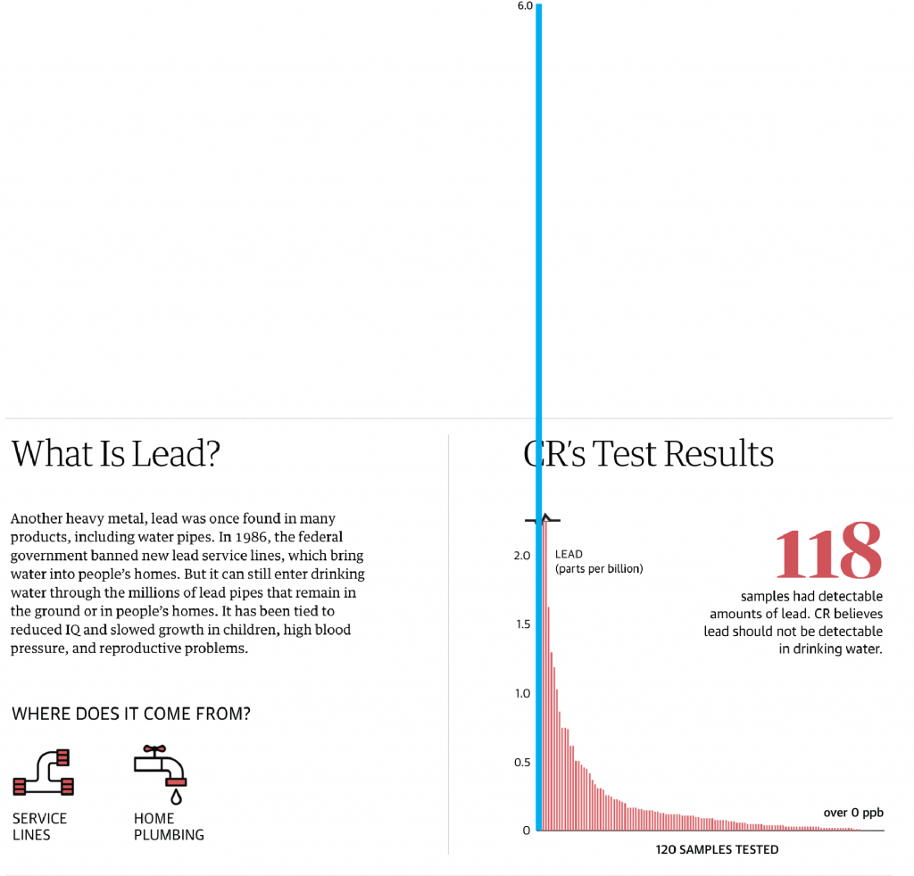
You can see that including the data point drastically changes how the chart looks. The number falls well outside the graphic, but it also shows just how dangerously high that one observation truly is.
But if you say, well yeah, but that falls outside the box allowed by the webpage, you’re correct. There are ways it could be handled to sit outside the “box”, but that would require some extra clever bits. And this isn’t a print layout where it’s much easier to play with placement. So what happens when we resize that graphic to fit within its container?
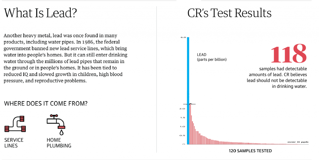
You can see that All the other bars become quite small. And this is probably why the designers chose to break the chart in the first place. But as we’ve established, in doing so they’ve minimised the danger of those few off-the-charts sites as well as left off context that shows how for the vast majority of sites, the situation is not nearly as dire—though, again, no lead is good lead.
What else could have been done? If maintaining the height of the less affected bars was paramount, the designers had a few other options they could have used. First, you could exclude those observations and perhaps put a line below the 118 text that says “for three sites, the data was off the charts and we’ve excluded them from the set below.”
I have used that approach in the past, but I use it with great reluctance. You are removing important outliers from the data set and the set is not complete without them. After all, if you are looking to use this data set to inform a policy choice such as, which communities should receive emergency funding to reduce lead levels, I’d want to start with the city in blue. Sure, I would like everyone to get money, but we’d have to prioritise resources.
I think the best compromise here would have actually been a small tweak to the original. Above the three bars that are broken (or perhaps to the right with some labelling), label the discontinuous data points to provide clearer context to the vast majority of the sites, which are below 0.5 ppb.
This preserves the ability to easily compare the lower level observations, but provides important context of where they sit within the overall data set by maintaining the upper limits of the worst offenders.
Credit for the piece goes to the Guardian’s graphics department.
Leave a Reply
You must be logged in to post a comment.