Datagraphic – Page 9 – Coffee Spoons

How the Globe’s Writers Voted

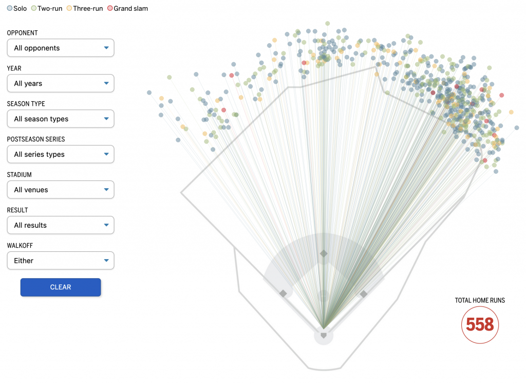
Yesterday we looked at a piece by the Boston Globe that mapped out all of David Ortiz’s home runs. We did that because he has just been voted into baseball’s Hall of Fame. But to be voted in means there must be votes and a few weeks after the deadline, the Globe posted an article about how that publication’s eligible voters, well, voted.

The graphic here was a simple table. But as I’ll always say, tables aren’t an inherently bad or easy-way-out form of data visualisation. They are great at organising information in such a way that you can quickly find or reference specific data points. For example, let’s say you wanted to find out whether or not a specific writer voted for a specific ballplayer.

Just don’t ask me for whom I would have voted…

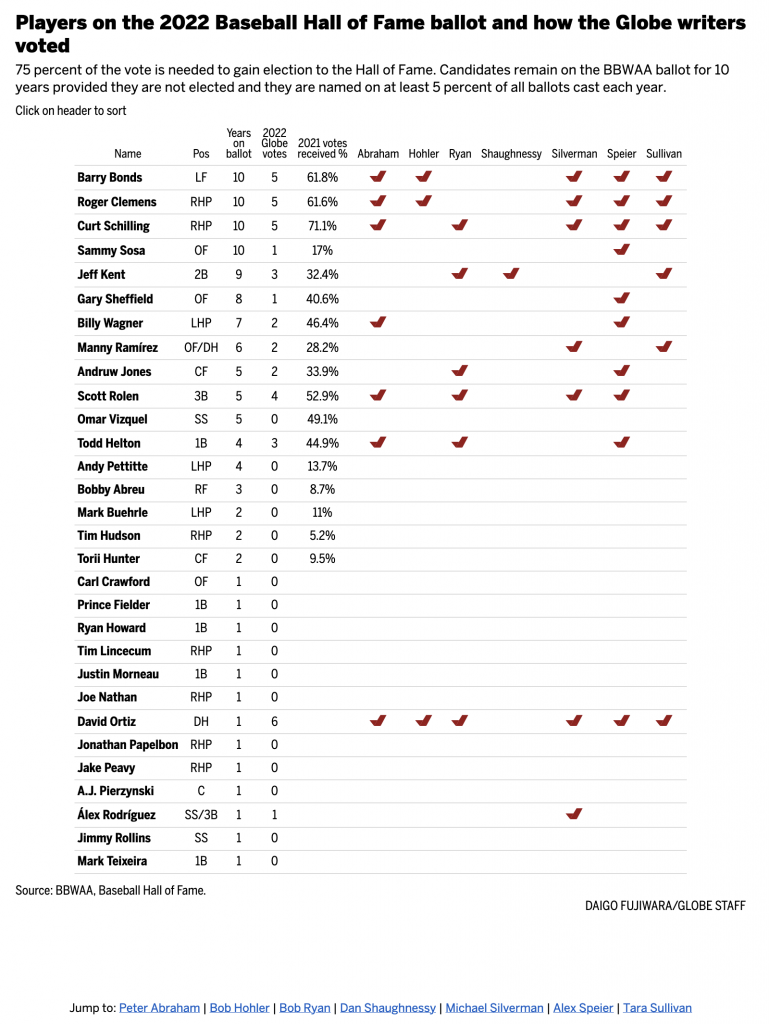
Simple red check marks represent those players for whom the Globe’s eligible staff voted. I really like some of the columns on the left that provide context on the vote. For the unfamiliar, players can only remain on the list for up to ten years. And so for the first four, this was their last year of eligibility. None made the cut. Then there’s a column for the total number of votes made by the Globe’s staff. Following that is more context, the share of votes received in 2021. Here the magic number if 75% to be elected. Conversely, if you do not make 5% you drop off the following year. Almost all of those on their first year ballot failed to reach that threshold.

The only potential drawback to this table is that by the time you reach the end of the table, there are few check marks to create implicit rules or lines that guide you from writer to player. David Ortiz’s placement helps because six—remarkably not all Globe writers voted for him—it grounds you for the only person below him (alphabetically) to receive a vote. And we need that because otherwise quickly linking Alex Rodriguez to Alex Speier would be difficult.

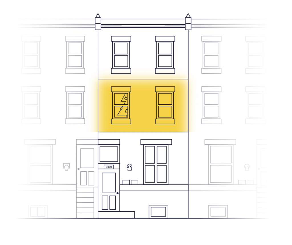
Finally below the table we have jump links to each writer’s writings about their selections. And if you’ll allow a brief screenshot of that…

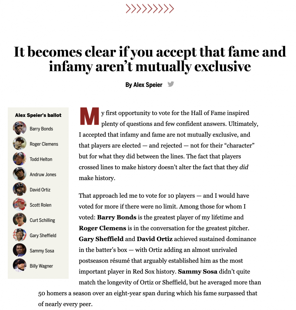
We have a nicely designed section here. Designers delineated each author’s section with red arrows that evoke the red stitching on a baseball. It’s a nice design tough. Then each author receives a headline and a small call out box inside which are the players—and their headshots—for whom the author voted. An initial dropped capital (drop cap), here a big red M, grabs the reader’s attention and draws them into the author’s own words.

Overall this was a solidly designed piece. I really enjoyed it. And for those who don’t follow the sport, the table is also an indicator of how divisive the voting can be. Even the Globe’s writers couldn’t unanimously agree on voting for David Ortiz.

Credit for the piece goes to Daigo Fujiwara and Ryan Huddle.

558 Dingers

Yesterday baseball writers elected David Ortiz of the Boston Red Sox, better known as Big Papi, to the Baseball Hall of Fame. I was trying to work on a thing for yesterday, but ran out of time. While I will attempt to return to that later, for now I want to share a simple interactive graphic from the Boston Globe. As the blog title suggests, it’s about the 558 career home runs Ortiz hit between his time with the Twins and the Red Sox. He hit 541 of those during the regular season, tacking on 17 more in the post season including his famous 2013 ALCS grand slam against the Detroit Tigers. (The one where the cop’s arms are in the air alongside Torii Hunter’s legs.)

Now you can see that Ortiz was a left-handed pull hitter with that home run concentration to right field, especially those wrapped around Fenway’s (in)famous Pesky Pole.

But with the number of dots you see inside the grounds at Fenway, you can also see the one downside of a chart like this. The graphic maps home runs at all Major League ballparks to that of Fenway. Not to mention the role that the Green Monster plays in turning a lot of those line drive home runs that when hit to right field leave the yard, but to left simply bounce off the Monster for doubles or the dreaded long single. But in part that’s why Ortiz also had ridiculous season numbers for extra base hits because of all those Green Monster doubles. (Conversely, how many popups a mile in the sky came down into the Green Monster seats?)

You access this interactive piece by scrolling through the experience as the Globe chose 12 home runs to represent Ortiz’s entire career. I’m fortunate enough to remember watching several of them on the television.

Big Papi was a force to be reckoned with and watching him hit was entertainment. I’m very excited to see him enter the Hall of Fame.

This summer? It’s his effing Hall.

Credit for the piece goes to John Hancock.

Finding Home with a Homemade Map

We’re going to start this week out with some good news and for that we turn to China. 30 years ago, child traffickers kidnapped four-year old Li Jingwei from his family and sold him to another family over 1,000 miles away. A BBC article from earlier this month covered Li Jingwei’s reunion with his family. How did it happen? Because of a map he drew and shared with the internet.

Here’s a screenshot of that map.

We all create mental maps of our surroundings. And not surprisingly they grow larger as we get older. But this man’s ability to recall details of his family hometown allowed internet sleuths, and eventually the police, to identify the village. DNA tests then connected Li to a woman whose son had been abducted.

When we draw out these maps ourselves they become a link to the cartographic world. And that this man was able to use his own mental map to find his home. Well, like I said, we’re going to start the news off with some good news.

Credit for the piece goes to Li Jingwei.

Tea. Earl Grey. Hot.

Any science fiction fan—and likely many who are not—can identify the character who utters those words in that order: Jean-Luc Picard, Star Trek’s captain of the USS Enterprise, NCC-1701-D. Ask your Amazon Alexa for it. Or your Google Home.

Thanks to the work of xkcd, we now know that Jean-Luc—may I call him Jean-Luc?—had a number of other options in the replicator from which to choose before he settled on “hot”.

Although Garak would still like to meet that Earl Grey and tell him a thing or two about tea leaves.

Credit for the piece goes to Randall Munroe.

Even Older Family Trees

Yesterday we looked at a graphic about an old family tree, revealed by ancient DNA. But at the end of the day it is a family tree of descent for a human male. But mankind itself fits within a kind of family tree, the ~~circle~~ family tree of life.

The tree of life continues to evolve as we discover new species and then reconfigure what we have to fit what we now know. When I was a wee lad in school, we learned about the three kingdoms of life: plants, animals, and fungi. Bacteria were a separate branch.

A few weeks ago, however, I was reading an article about how a recent DNA analysis identified a new “supergroup” within our larger group of complex cellular life, eukaryotes (plants, animal, and fungi fall within this). Luckily for our purposes the article contains a small graphic at which we can take a look.

Humans are way, way, way down on the tree.

The diagram uses a fairly simple design. Two panels split the largest groupings into its branches whilst the second panel breaks up eukaryotes. Colour links the eukaryotes together and shows how they fit into the broader tree to the left, which uses dark grey and light blue for bacteria and archaea, respectively.

A nice additional touch was the designer’s decision to include a small icon that represents the name of the supergroups within eukaryotes. Because, as the text points out, we don’t have commonly known names for these supergroups. Did I know that we belong to the opisthokonts? Absolutely not. Although dog people may be upset that the cat got the call to represent animals.

Regardless of the design, you can still see in the second panel how people are more closely related to amoeba than we are plants. But this new supergroup, hemimastigotes, branches off from the rest of us eukaryotes at a very early point. And the DNA proves it.

Overall this was a really nice graphic to see in a fascinating article. Science is cool.

Credit for the piece goes to Lucy Reading-Ikkanda.

Old Family Trees

Another quick little post from a little while back, around Christmas news broke about the oldest family tree yet discovered. Researchers used DNA recovered from a 5700-year old tomb in the UK to piece together the relationships between the people interred within the tomb.

Graphic wise, we’re not talking about anything crazy or inventive here—it’s a family tree after all. But the designers did a nice job using colour to indicate the different family groups of descent, which were spatially organised within the tomb by the woman to whom the children were born. To be fair, it was all based upon the descendants of one man, but one man who had several wives.

What’s fascinating about this, however, is simply the age. We can go back nearly 6,000 years and simply from DNA create a family tree five generations deep.

The only thing I wish is that we had an accompanying map of the tomb, because that’s the other key part of the story. But at the end of the day I’ll always take a nice family tree.

Credit for the piece goes to Newcastle University’s design team.

Showing All 50

Those who know me know one of my pet peeves are when maps of the United States do not display Alaska and Hawaii. I even noted yesterday that those two states were so late of additions to the United States and it made sense as to why they were not included.

So when I was going through some old photos yesterday, I stumbled across this of a poster on the Philadelphia subway system. I had flagged it for posting, but I guess I never did.

I understand this is an advert and so for creative purposes, creative liberty. And it could be that this service does not exist in either Alaska or Hawaii.

But, the statement here is that Metro covers 99% of the United States. Geographically, to do so Metro must cover Alaska because in terms of land area, Alaska comprises nearly 18% of the entire United States. Yeah, Alaska is big. Now, if you’re talking covering 99% of the people of the United States, Metro has some wiggle room. Combined, both Alaska and Hawaii comprise 0.6% of the United States population. That would still leave 0.4% of the American population not covered, and by definition that must be some part of the contiguous lower 48. But above we can see the whole map is purple.

In other words, this is not an accurate map. They should have found some way of incorporating Alaska and Hawaii.

Credit for the piece goes to Metro’s designer or design agency.

Slaveholders in the Halls of Congress

Taking a break from going through the old articles and things I’ve saved, let’s turn to a an article from the Washington Post published earlier this week. As the title indicates, the Post’s article explores slaveholders in Congress. Many of us know that the vast majority of antebellum presidents at one point or another owned slaves. (Washington and Jefferson being the two most commonly cited in recent years.) But what about the other branches of government?

The article is a fascinating read about the prevalence of slaveholders in the legislative branch. For our purposes it uses a series of bar charts and maps to illustrate its point. Now, the piece isn’t truly interactive as it’s more of the scrolling narrative, but at several points in American history the article pauses to show the number of slaveholders in office during a particular Congress. The screenshot below is from the 1807 Congress.

That year is an interesting choice, not mentioned explicitly in the article, because the United States Constitution prohibited Congress from passing limits on the slave trade prior to 1808. But in 1807 Congress passed a law that banned the slave trade from 1 January 1808, the first day legally permitted by the Constitution.

Almost half of Congress in the early years had, at one point or another, owned slaves.

Graphic-wise, we have a set of bar charts representing the percentage and then a choropleth map showing each state’s number of slaveholders in Congress. As we will see in a moment, the map here is a bit too small to work. Can you really see Delaware, Rhode Island, and (to a lesser extent) New Jersey? Additionally, because of the continuous gradient it can be difficult to distinguish just how many slaveholders were present in each state. I wonder if a series of bins would have been more effective.

The decision to use actual numbers intrigues me as well. Ohio, for example, has few slaveholders in Congress based upon the map. But as a newly organised state, Ohio had only two senators and one congressman. That’s a small actual, but 33% of its congressional delegation.

Overall though, the general pervasiveness of slaveholders warrants the use of a map to show geographic distribution was not limited to just the south.

Later on we have what I think is the best graphic of the article, a box map showing each state’s slaveholders over time.

How the trends changed over time over geography.

Within each state we can see the general trend, including the legacy of the Civil War and Reconstruction. The use of a light background allows white to represent pre-statehood periods for each state. And of course some states, notably Alaska and Hawaii, joined the United States well after this period.

But I also want to address one potential issue with the methodology of the article. One that it does briefly address, albeit tangentially. This data set looks at all people who at one point or another in their life held slaves. First, contextually, in the early years of the republic slavery was not uncommon throughout the world. Though by the aforementioned year of 1807 the institution appeared on its way out in the West. Sadly the cotton gin revolutionised the South’s cotton industry and reinvigorated the economic impetus for slavery. There after slavery boomed. The banning of the slave trade shortly thereafter introduced scarcity into the slave market and then the South’s “peculiar institution” truly took root. That cotton boom may well explain how the initial decline in the prevalence of slaveholders in the first few Congresses reversed itself and then held steady through the early decades of the 19th century.

And that initial decline before a hardening of support for slavery is what I want to address. The data here looks only at people who at one point in their life held slaves. It’s not an accurate representation of current slaveholders in Congress at the time they served. It’s a subtle but important distinction. The most obvious result of this is how after the 1860s the graphics show members of Congress as slaveholders when this was not the case. They had in the past held slaves.

That is not to say that some of those members were reluctant and, in all likelihood, would have preferred to have kept their slaves. And therefore those numbers are important to understand. But it undermines the count of people who eventually came to realise the error of their ways. The article addresses this briefly, recounting several anecdotes of people who later in life became abolitionists. I wonder though whether these people should count in this graphic as—so far as we can tell—their personal views changed so substantially to be hardened against slavery.

I would be very curious to see these charts remade with a data set that accounts for contemporary ownership of slaves represented in Congress.

Regardless of the methodology issue, this is still a fascinating and important read.

Credit for the piece goes to Adrian Blanco, Leo Dominguez, and Julie Zuazmer Weil.

Fire in Fairmount

Philadelphia made the national and international news last week, although for once not because we’re all being shot to death. This time because a fire in a rowhome killed 12 people, including nine children. The Philadelphia Inquirer quickly posted a short article explaining what occurred that morning. But the early indication, based upon the confession of a five-year old, is that a child playing with a light set a live Christmas tree on fire.

Ironically, the city prohibits live trees in high rises, apartment buildings, and multi-family dwellings. The rule is in place because live trees are a very real fire hazard. Just a few weeks earlier, a man and two of his sons were killed in a suburb north of Philadelphia (his wife and a third son survived). They died in a fire that began with lights on a live tree. But here in the city, the code states that multi-family dwellings begin at three households. This rowhome had been converted into two separate units, so a live tree was legal. But they would have been better without.

The Inquirer article features a scrolling illustration depicting what we presently know about the fire: how and where it started, why it may have spread, and ultimately who died.

Live trees smell great, but they’re a very real fire risk.

Credit for the piece goes to Sam Morris.

Space: The Final Frontier

We’re back after a nice holiday break. And one of the most fascinating things to happen was the successful—and seemingly easy, more on that in a bit—launch of the James Webb space telescope. The James Webb was developed by NASA with contributions from both the European Space Agency (ESA) and the Canadian Space Agency (CSA). Whilst it did launch behind schedule and at a price tag of $10 billion, the James Webb is the most sophisticated and complex space telescope mankind has yet launched into space. It will look backwards into time to some of the earliest stars and galaxies in the universe. It will also look at the thousands of exoplanets we have discovered in the last three decades. The instruments aboard James Webb will be able to help us identify if any of these planets have water and other ingredients necessary for life as we know it. This could be one of the most monumental space missions yet.

But James Webb’s launch was far from guaranteed. As this great article from the BBC explains, the construction, assembly, launch, and deployment were all incredibly complicated. James Webb is expected to operate for ten years before its fuel, needed to keep the telescope cold, runs out. However, the seemingly easy launch and deployment means that it used less fuel than expected. Some early reports suggest that the telescope may have some additional time left in it now before the fuel runs dry.

I encourage you to read the article, because it explains the advantages of the telescope, how it works, and its deployment with several illustrations. There are five in particular, though I’ll share only two screenshots.

The most important is this, the key distinction between Hubble and James Webb. It shows how the two space telescopes will be operating in different parts of the electromagnetic spectrum.

The graphic fakes the colours, because by definition we can only see the visible portions of the spectrum. Wavelengths get either too short or too long on either side of the visible spectrum—which differs for different species. I would actually really enjoy seeing how these two spectra stack up against other space observatories like Chandra (x-ray) and Spitzer (infrared).

Next we have the deployment, which finished just last week. The graphic summarises how complicated this process was—and how fraught with risk. But in the end it went off without any major hitch.

Make sure to read the instructions before deployment…

This uses a nice series of small multiples of illustrations. These simplified drawings show how the tightly packed telescope unfolds and then begins deploying its vital heat shield then its mirror.

The last thing to check out in the article is a slider showing the “before” and “after”. You have seen them before for things like flood or hurricane damages. Here, however, you can compare a photo in Hubble’s visible light to an existing infrared version of the same photo.

Of course, just because the telescope finished deploying its mirror last week doesn’t mean we get photos this week. The Baltimore-based team running the observatory will spend the next few months tuning everything up. But the goal is hopefully to have the first images from James Webb sometime in June.

And then we have the next ten years to hopefully start collecting data.

Credit for the piece goes to the BBC graphics team.