Tag: small multiples
-
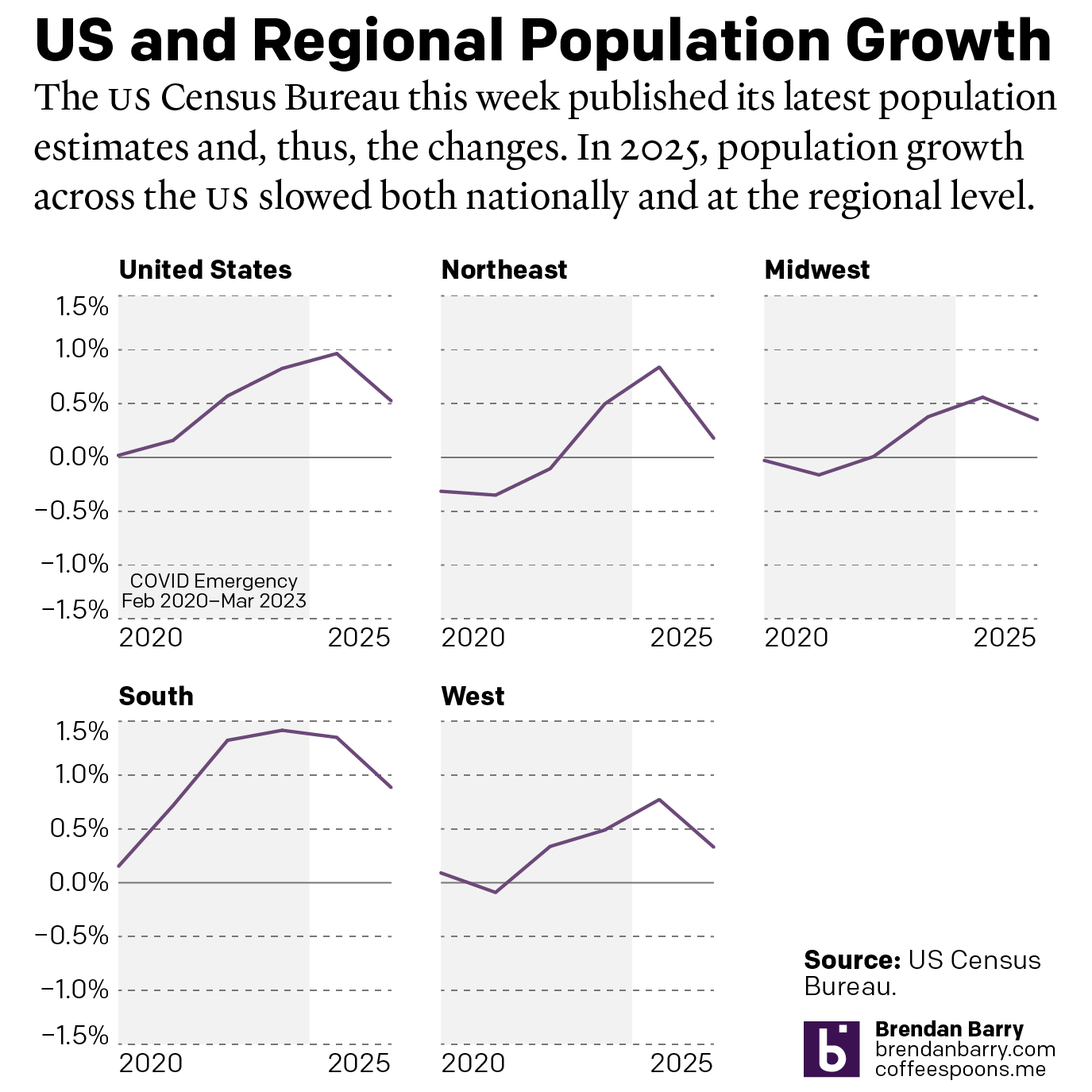
The Slowing of the Growth
This week the US Census Bureau released their population estimates for the most recent year and that includes the rate changes for the US, the Census Bureau defined regions, and the 50 states and Puerto Rico. I spent this morning digging into some of the data and whilst I will try to later to get…
-
Bridging the Difference
When I was a wee lad, I entered the school science fair and made models of different types of bridges. Suspension, cantilever, &c. I saw this a little while back and bookmarked it. As I am trying to get back into the swing of publishing here on Coffee Spoons, it’s time to bring back the…
-
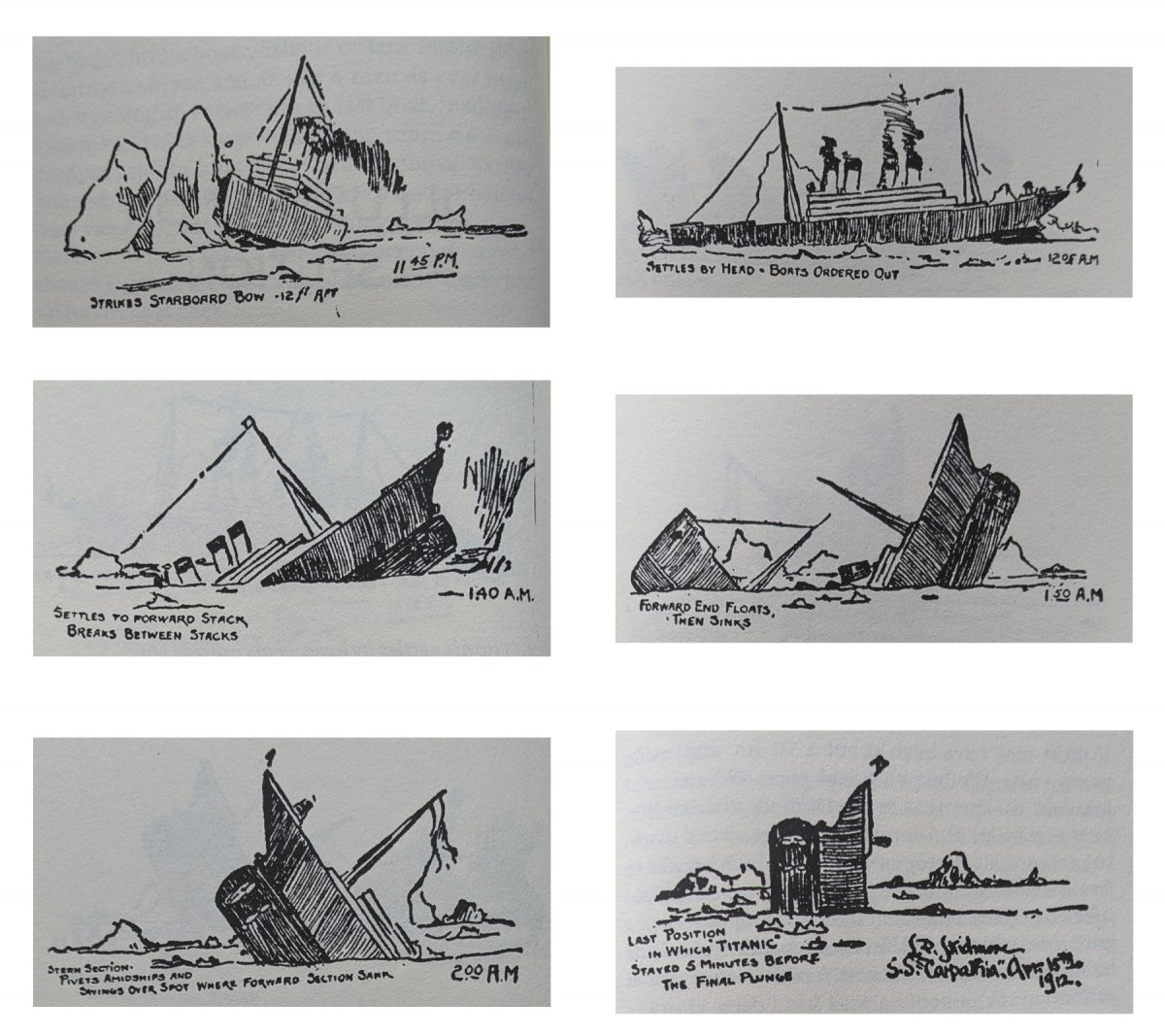
Illustrating the Sinking of RMS Titanic
After all the years of writing and publishing here on Coffeespoons, content centred on the sinking of RMS Titanic remains the most popular. And it was in the early hours of 15 April 1912 when she slipped beneath the surface of the North Atlantic. 700 people survived. 1500 people did not. Titanic’s sinking was the…
-
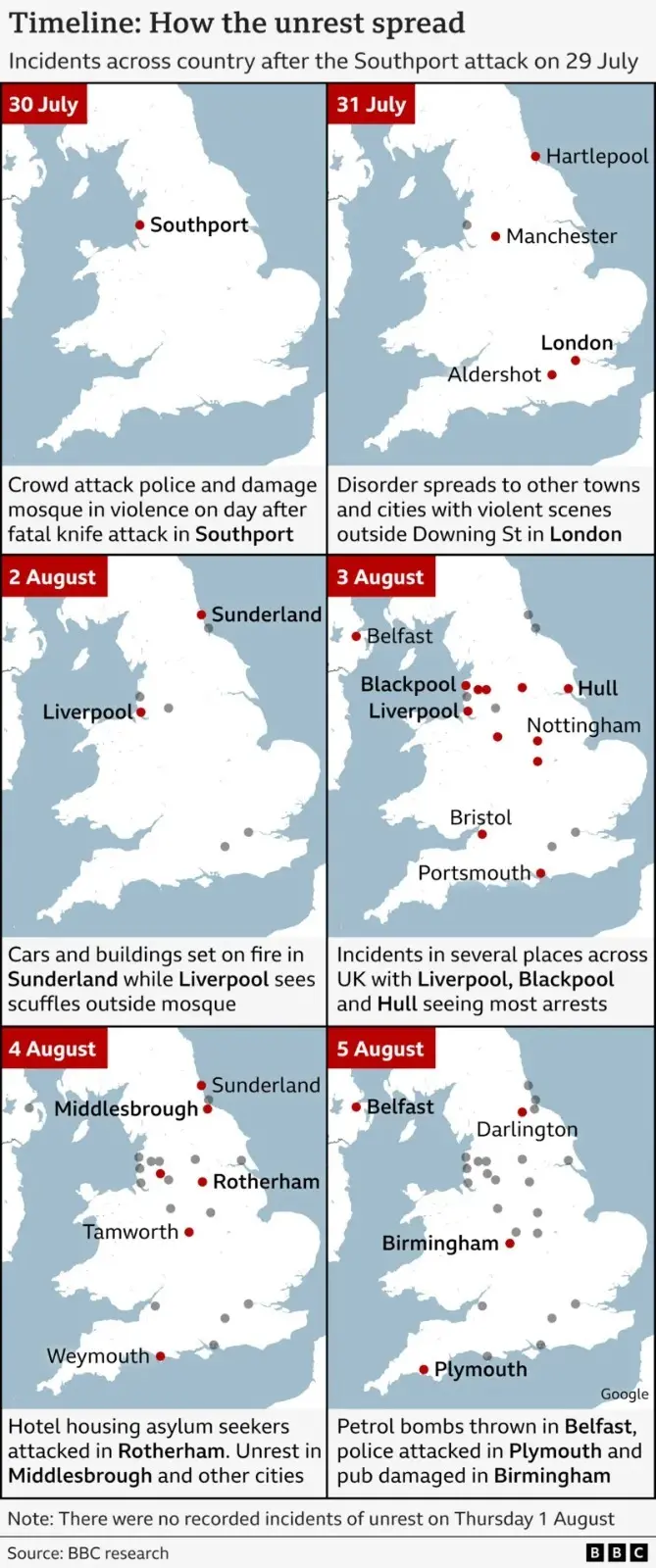
I Didn’t Predict a Riot
Yesterday I wrote about a BBC graphics locator map that was perhaps not as helpful as possible. Well today I want to talk about another BBC map, though not in as critical a fashion. I landed upon this map whilst reading a series of updates about last month’s anti-immigrant riots throughout the United Kingdom—principally England.…
-
Warming Towards Women Leaders
We are going to start this week off with a nice small multiple graphic that explores the reducing resistance to women in positions of leadership in Arab countries. The graphic comes from a BBC article published last week. These kinds of graphics allow a reader to quickly compare the trajectory of a thing between a…
-
Space: The Final Frontier
We’re back after a nice holiday break. And one of the most fascinating things to happen was the successful—and seemingly easy, more on that in a bit—launch of the James Webb space telescope. The James Webb was developed by NASA with contributions from both the European Space Agency (ESA) and the Canadian Space Agency (CSA).…
-
Back to the Office, Back to Basics
Two weeks ago I posted about an article from the BBC that used graphics about which I was less than thrilled. Inconsistent use of axis lines, centring the graphic were two of the things that irked me. Two weeks hence, I do want to draw some positive attention to another article in the BBC. This…
-
The Month That Lasted a Year
Two Fridays ago I received my second dose of the vaccine. In other words, I’m fully vaccinated and can resume doing…things. Anything. And so this piece from xkcd seemed an appropriate way to wrap up what has been a horrible, no good, terrible year. Credit for the piece goes to Randall Munroe.