Today is yet another Friday in the pandemic. And so I wanted to just upload a few of the graphics I have been making for family, friends, and coworkers and posting on the Instagram and the Facebook. I did this two weeks ago as well, and if you compare those maps to these, you will see quite a stark difference. But on to today’s maps.
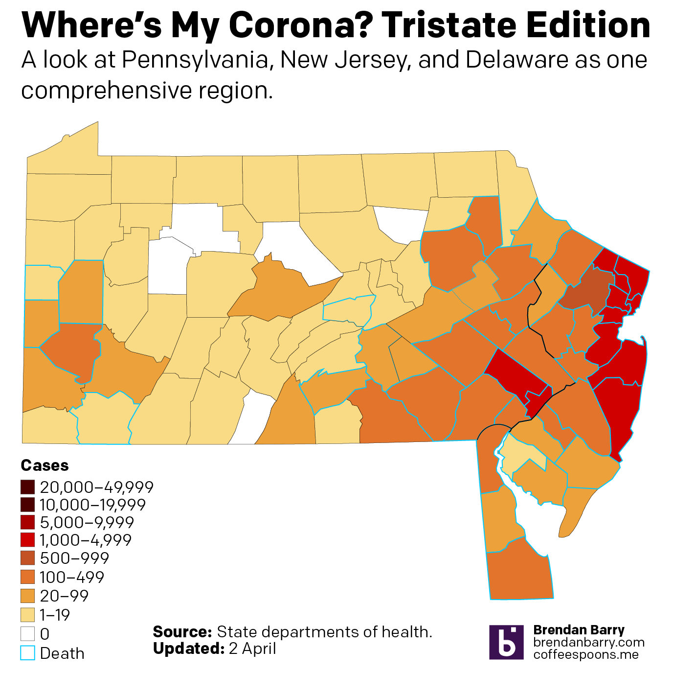
As a brief reminder, I am specifically looking at Pennsylvania, New Jersey, and Delaware—the tri-state region for my non-Philly followers—as well as Virginia and Illinois by the request of friends and former colleagues who live in those states. And then at the end I’ve been putting the tri-state region together to provide a fuller regional context.
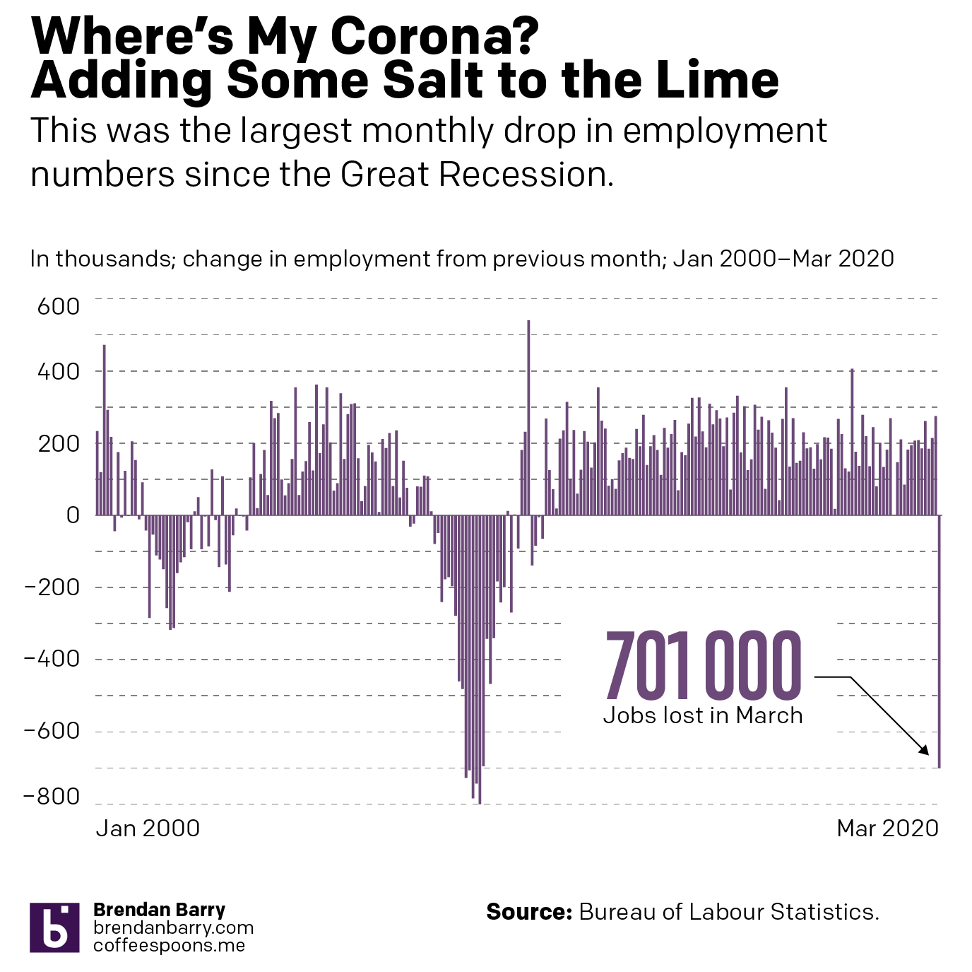
Lastly, for today only, the Bureau of Labour Statistics published its jobs report about the number of job losses in March across the US. And…it wasn’t pretty.
Conditions in PennsylvaniaConditions in New JerseyConditions in DelawareConditions in VirginiaConditions in IllinoisConditions in the tri-state region
Plus, the added bonus of the Bureau of Labour Statistics’ monthly jobs report. And spoiler, things aren’t so great out there.
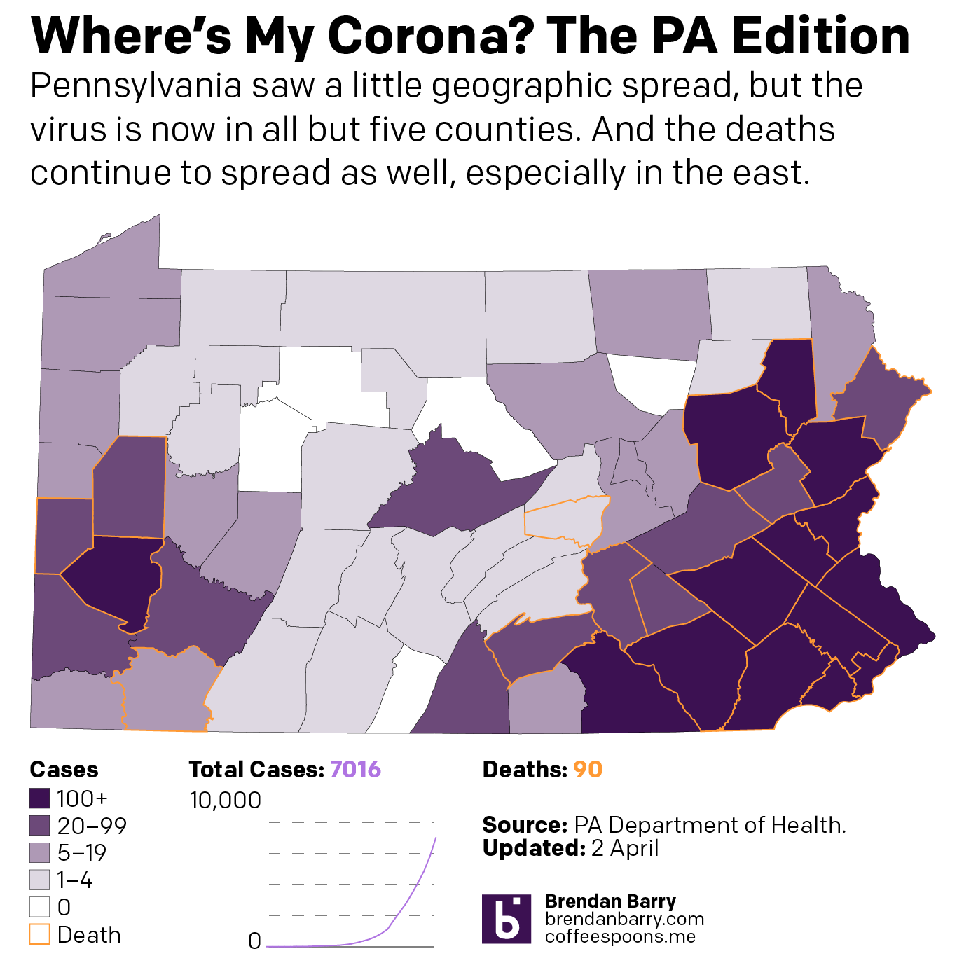
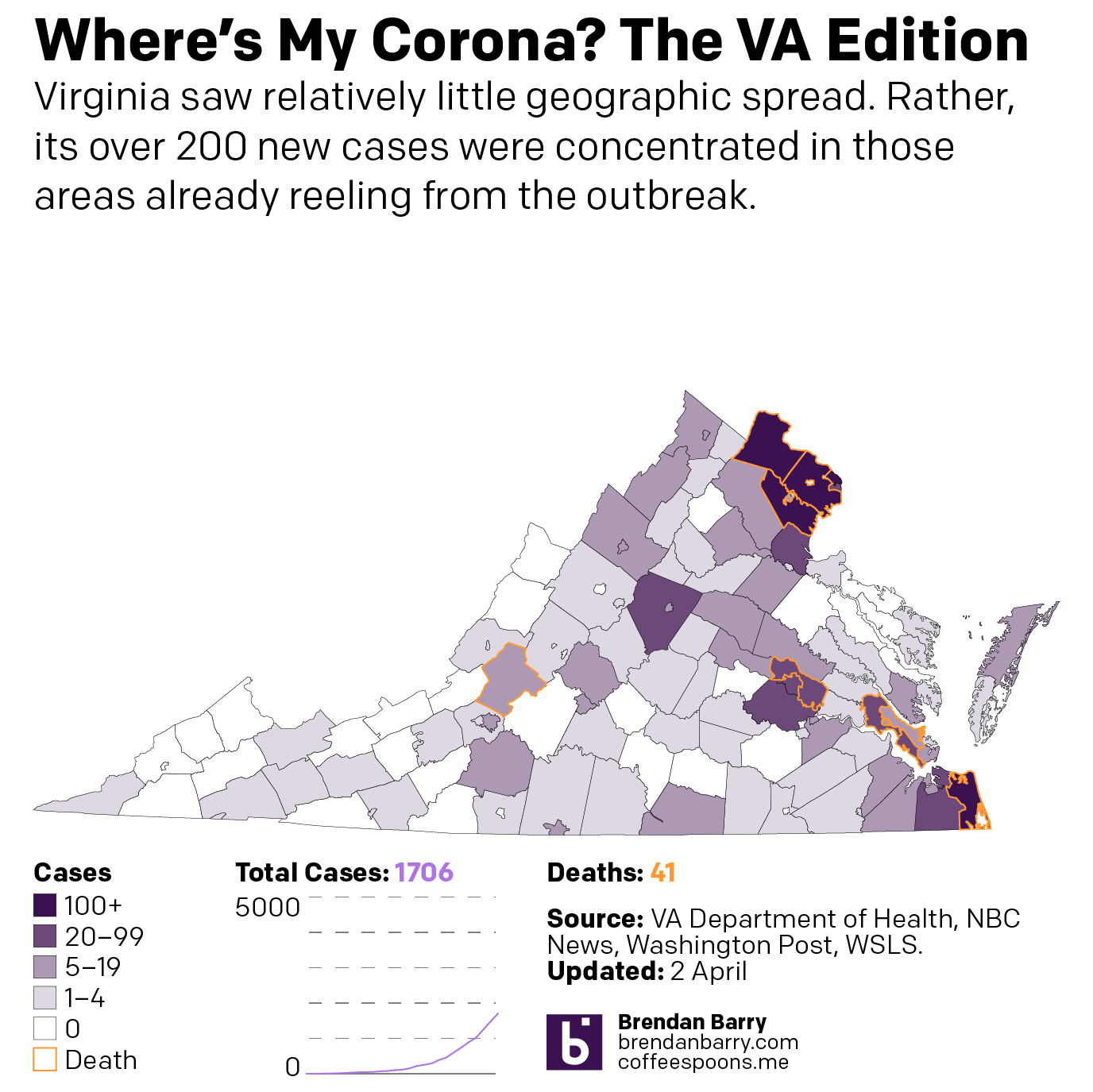
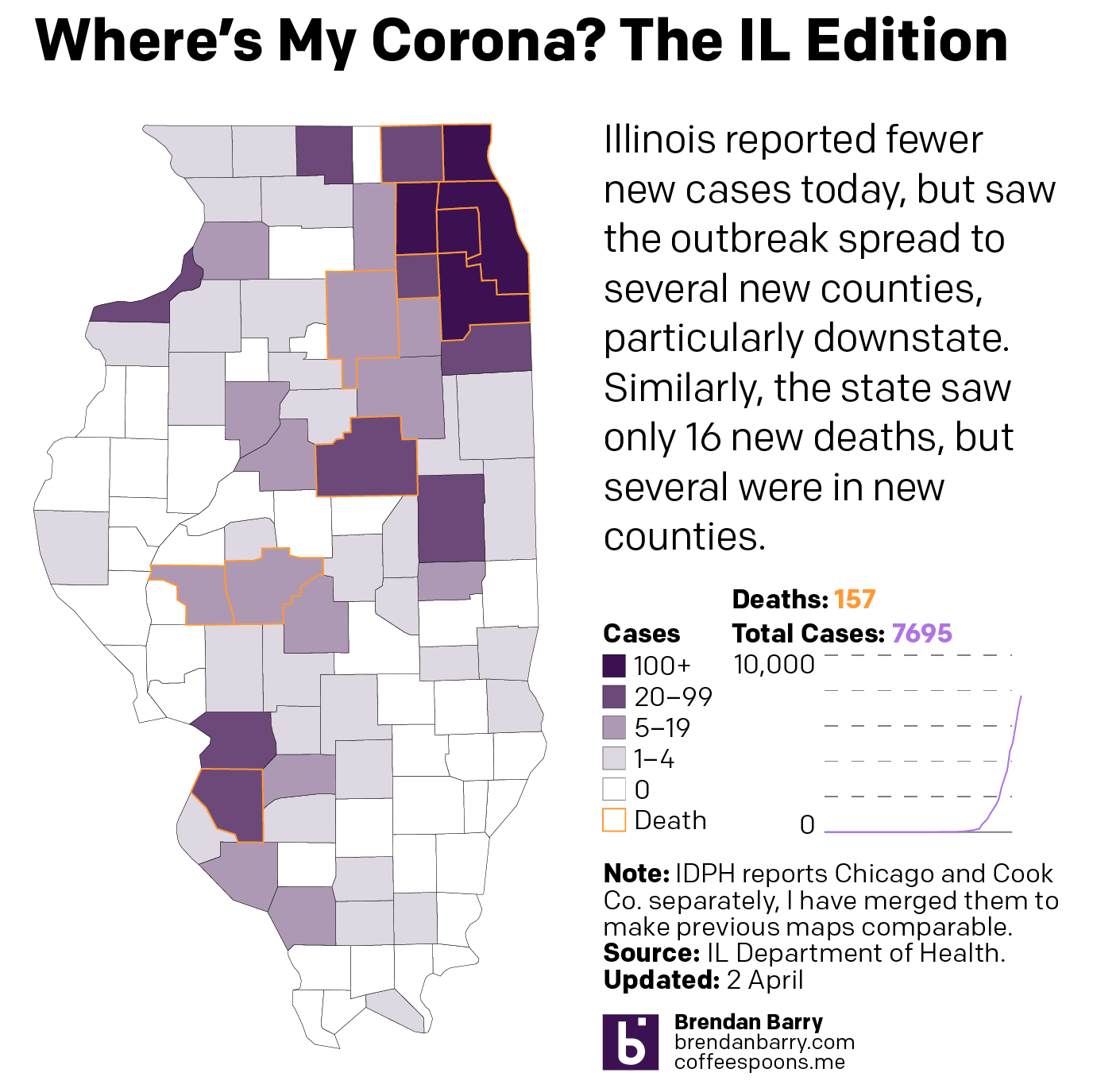
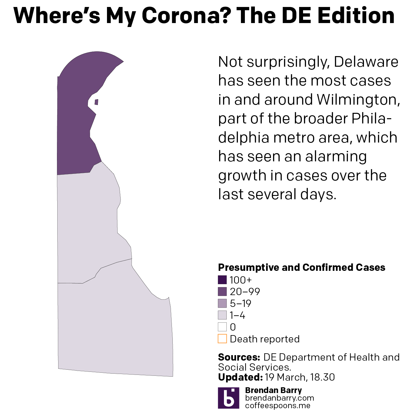
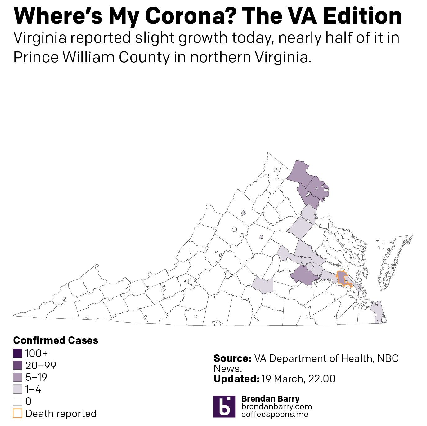
By now we have probably all seen the maps of state coverage of the COVID-19 outbreak. But state level maps only tell part of the story. Not all outbreaks are widespread within states. And so after some requests from family, friends, and colleagues, I’ve been attempting to compile county-level data from the state health departments where those family, friends, and colleagues live. Not surprisingly, most of these states are the Philadelphia and Chicago metro areas, but also Virginia.
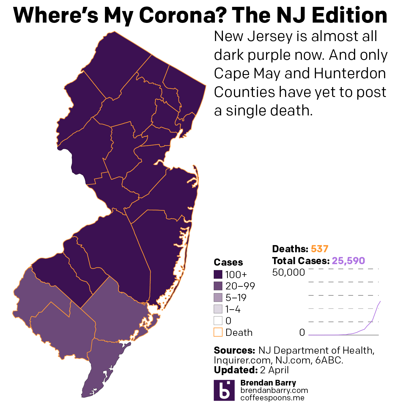
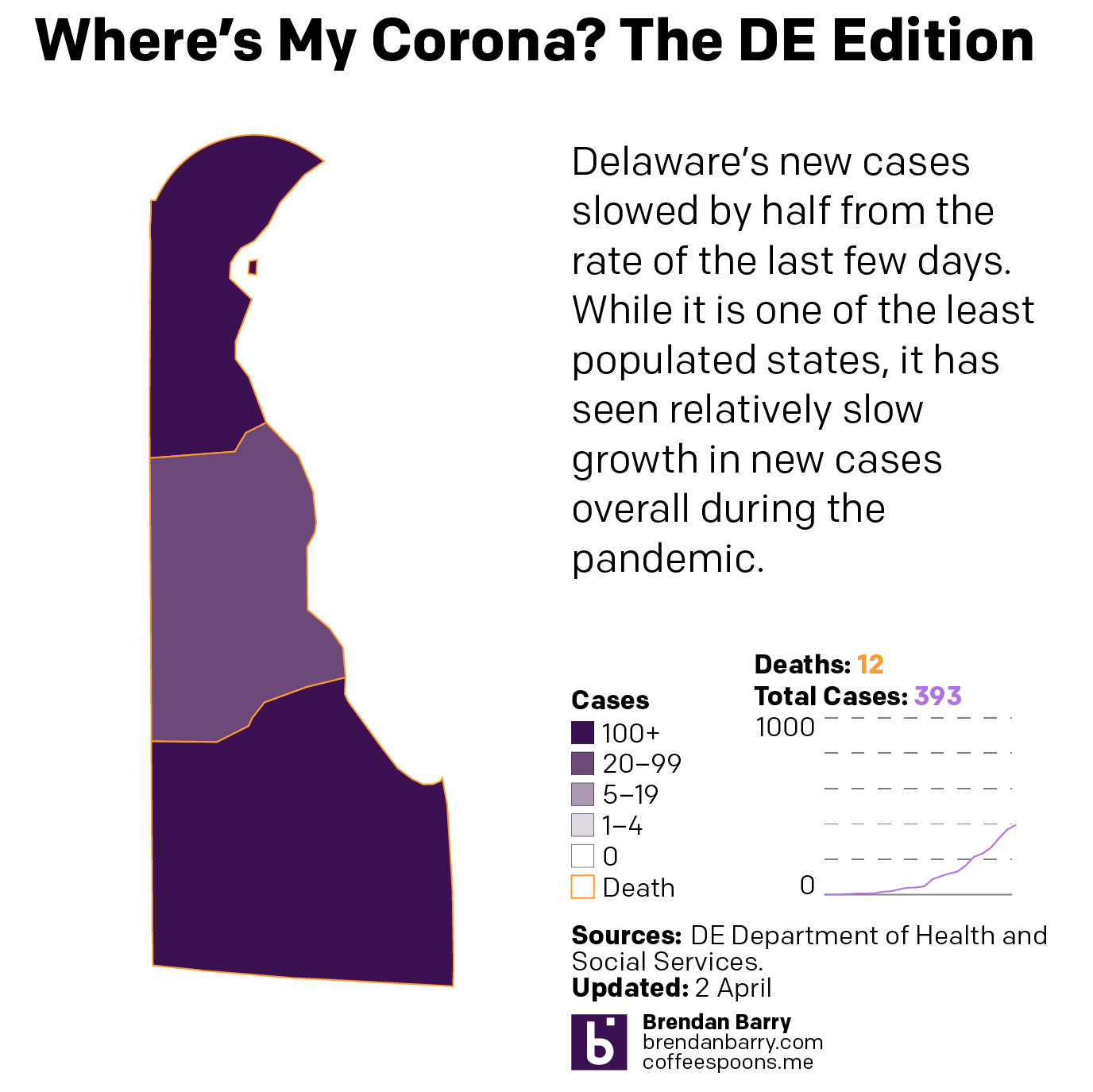
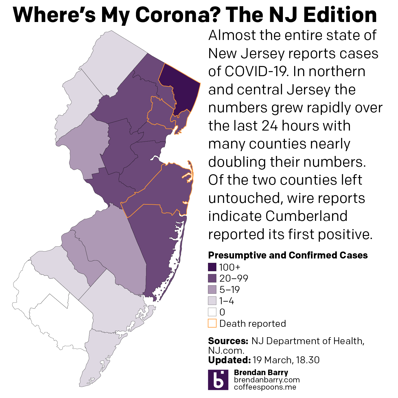
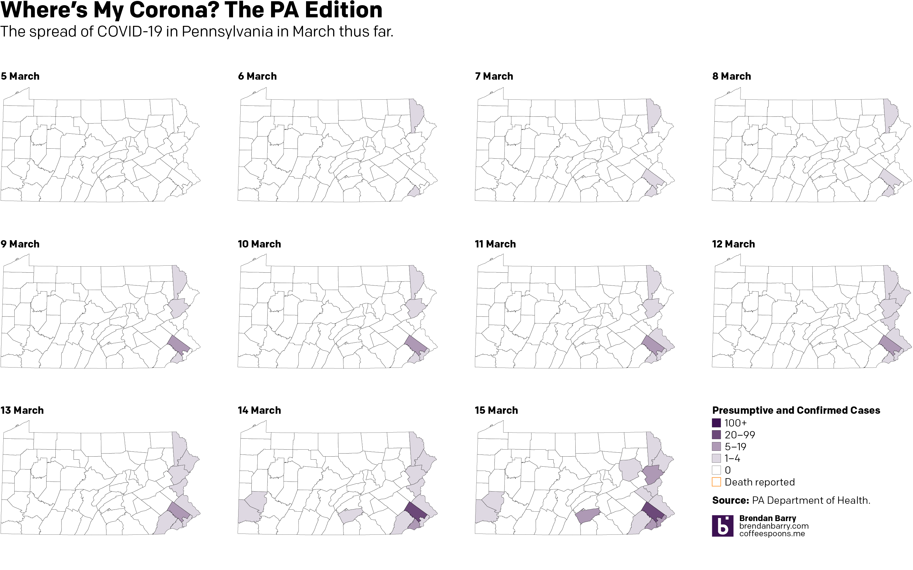
These are all images I have posted to Instagram. But the content tells a familiar story. The outbreaks in this early stage are all concentrated in and around the larger, interconnected cities. In Pennsylvania, that means clusters around the large cities of Philadelphia, Pittsburgh, and Harrisburg. In New Jersey they stretch along the Northeast Corridor between New York and Trenton (and along into Philadelphia) and then down into Delaware’s New Castle County, home to the city of Wilmington. And then in Virginia, we see small clusters in Northern Virginia in the DC metro area and also around Richmond and the Williamsburg area. Finally in Illinois we have a big cluster in and around Chicago, but also Springfield and the St. Louis area, whose eastern suburbs include Illinois communities like East St. Louis.
19 March county wide spread of COVID-1919 March county wide spread of COVID-1919 March county wide spread of COVID-1919 March county wide spread of COVID-1919 March county wide spread of COVID-19
I have also been taking a more detailed look at the spread in Pennsylvania, because I live there. And I want to see the rapidity with which the outbreak is growing in each county. And for that I moved from a choropleth to a small multiple matrix of line charts, all with the same fixed scale. And, well, it doesn’t look good for southeastern Pennsylvania.
County levels compared
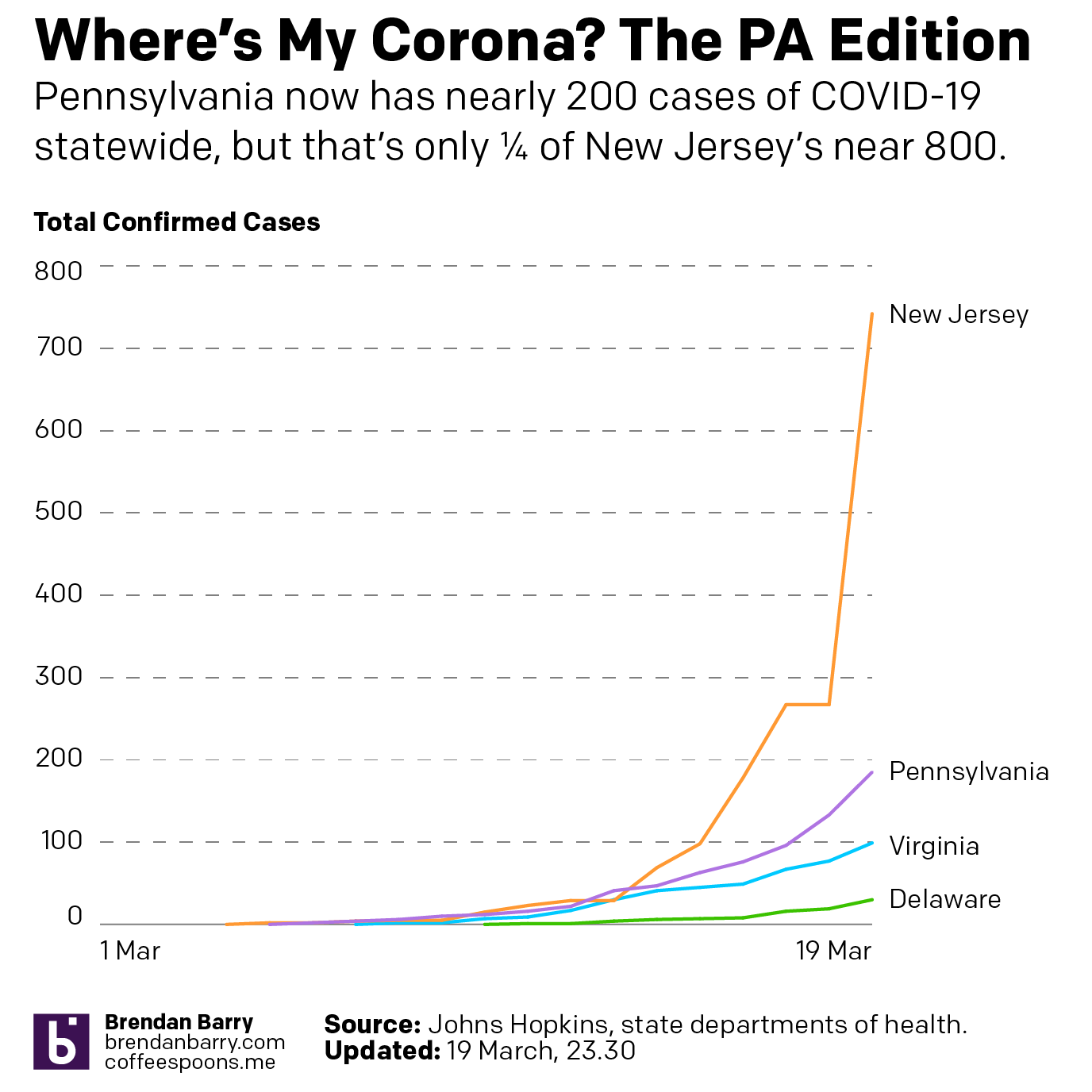
Then last night I also compared the total number of cases in Pennsylvania, New Jersey, Delaware, and Virginia. Most interestingly, Pennsylvania and New Jersey’s outbreaks began just a day apart (at least so far as we know given the limited amount of testing in early March). And those two states have taken dramatically different directions. New Jersey has seen a steep curve doubling less than every two days whereas Pennsylvania has been a bit more gradual, doubling a little less than every three.
State levels since early March
For those of you who want to continue following along, I will be looking at potential options this coming weekend whilst still recording the data for future graphics.
Over the last several days, along with most of the country, I’ve taken an interest in the spread of the novel coronavirus named COVID-19. Though, to be fair, it’s actually been in the news since early January, though early news reports like this from the Times, simply called it a mysterious new virus. At the time I thought little of it, because the news out of China was that it did not appear it could spread amongst humans. How did that idea…wait for it…pan out?
Anyway, over the last couple of days I’ve been making some maps for Instagram because people tend to look at a national map and see every nearly state infected when, in reality, there are pockets and clusters within those states. So I started looking at Pennsylvania. And initially, the cluster was along the Delaware River, namely Pennsylvania as well as its upper reaches near the Lehigh Valley and in the far northeast of the state.
But the spread has grown, and fairly quickly, with Montgomery County, a Philadelphia suburb, a hotspot. Consequently, the Pennsylvania governor has shut down all schools across the state and ordered non-essential shops, restaurants, and bars in the counties surrounding Philadelphia—as well as the county containing Pittsburgh—closed.
So 11 days in, here’s where we stand. (To be fair, I looked at including the early numbers out of today, but nothing has really changed, so I’ll wait until the evening figures are released before I update this again.)
Credit is mine. Data is the Pennsylvania Department of Health.
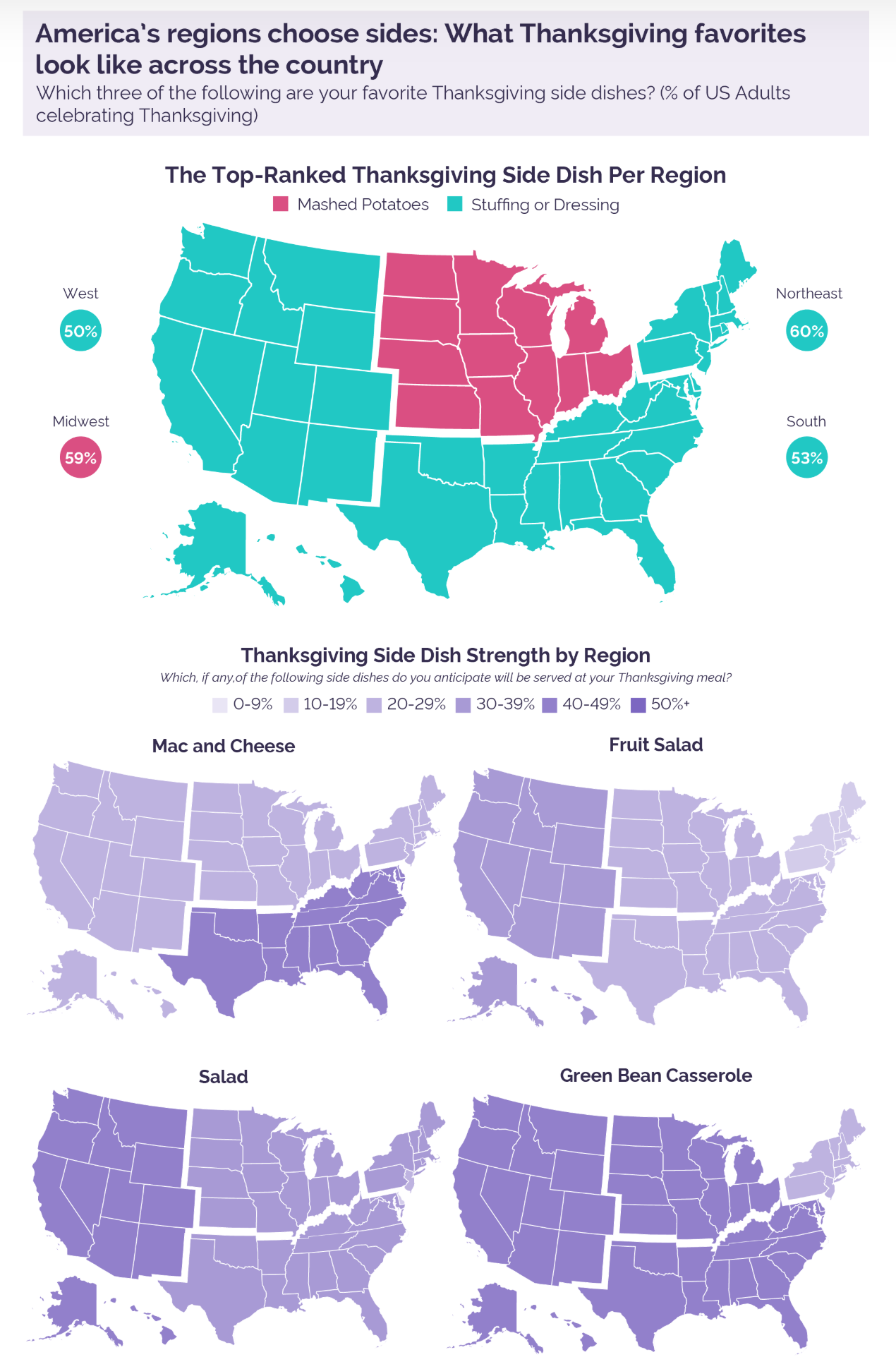
American Thanksgiving meals often feature elaborate spreads of side dishes. And everyone has a favourite. A common theme around the holiday is for media outlets to conduct surveys to see which ones are most popular where. In today’s piece we have one such survey from pollster YouGov. In particular, I wanted to focus on a series of small multiples maps they used to illustrate the preferences.
Big splashes of colour do not necessarily make for a great map
I used to see this approach taken more often and by this I hope I do not see a foreshadow of its comeback. Here we have US states aggregated into distinct regions, e.g. the Northeast. One could get into an argument about how one defines what region. The Midwest is one often contested such region—I have one post on it dating back to at least 2014.
Instead, however, I want to focus on the distinction between states and regions. This small multiples graphic is a set of choropleth maps that use side dish preferences to colour the map. Simple enough. However, the white lines delineating states imply different fields to be coloured within the graphic. Consequently, it appears that each state within the region has the same preference at the same percentage.
The underlying data behind the maps, at least that which was released, indicates the data is not at the state level but instead at the regional level. In other words, there are no differences to be seen between, say, Pennsylvania and New Jersey. Consequently, a more appropriate map choice would have been one that omitted the state boundaries in favour of the larger outlines of the regions.
More radically, a set of bar charts would have done a better job. Consider that with the exception of fruit salad, in every map, only one region is different than the others. A bar chart would have shown the nuance separating the three regions that in almost all of these maps is lost when they all appear as one colour.
I appreciate what the designers were attempting to do, but here I would ask for seconds, as in chances.
Credit for the piece goes to the YouGov graphics team.
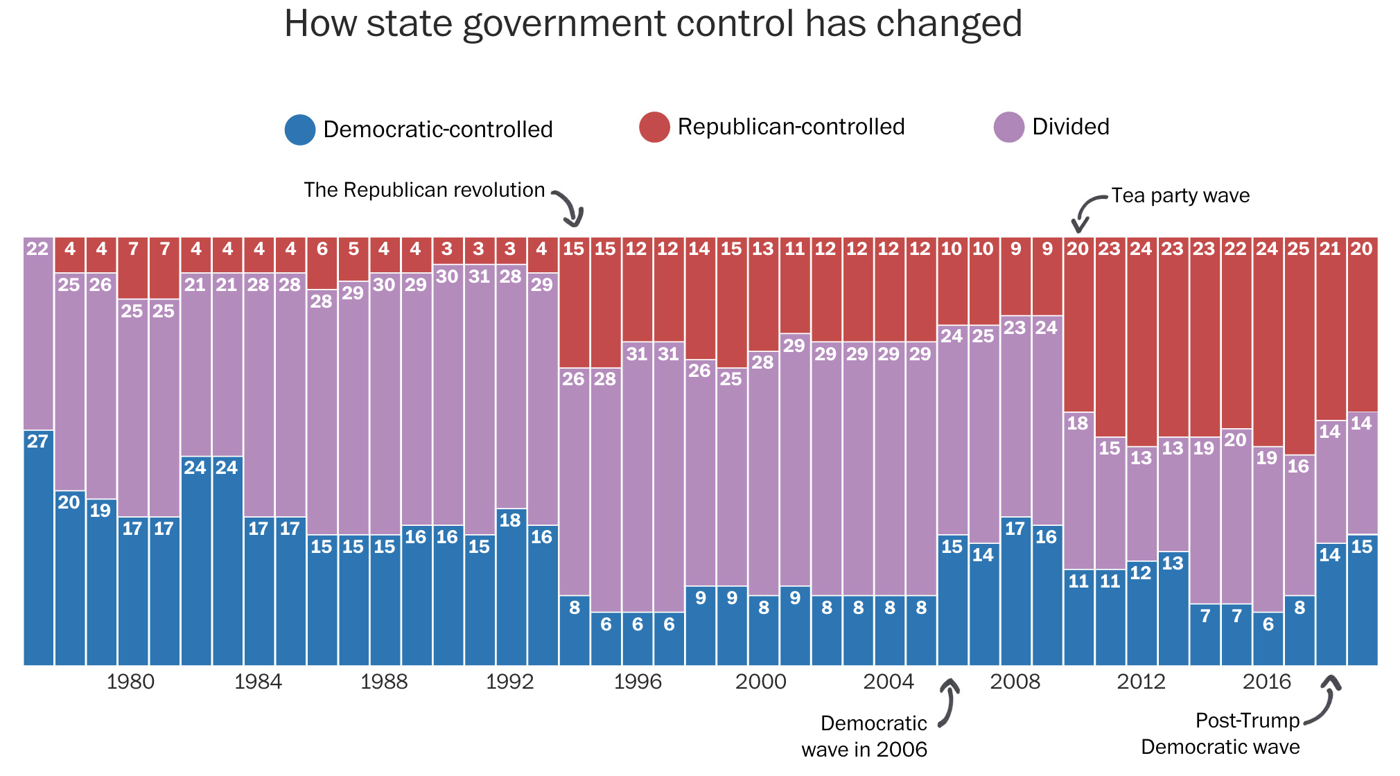
In a recent Washington Post piece, I came across a graphic style that I am not sure I can embrace. The article looked at the political trifecta at state levels, i.e. single political party control over the government (executive, lower legislative chamber, and upper legislative chamber). As a side note, I do like how they excluded Nebraska because of its unicameral legislature. It’s also theoretically non-partisan (though everybody knows who belongs to which party, so you could argue it’s as partisan as any other legislature).
At the outset, the piece uses a really nice stacked bar chart. It shows how control over the levers of state government have ebbed and flowed.
You can pretty easily spot the recent political eras by the big shifts in power.
It also uses little black lines with almost cartoonish arrowheads to point to particular years. The annotations are themselves important to the context—pointing out the various swing years. But from an aesthetic standpoint, I have to wonder if the casualness of the marks detracts from the seriousness of the content.
Sometimes the whimsical works. Pie charts about pizza pies or pie toppings can be whimsical. A graphic about political control over government is a different subject matter. Bloomberg used to tackle annotations with a subtler and more serious, but still rounded curve type of approach. Notably, however, Bloomberg at that time went for an against the grain, design forward, stoic business serious second approach.
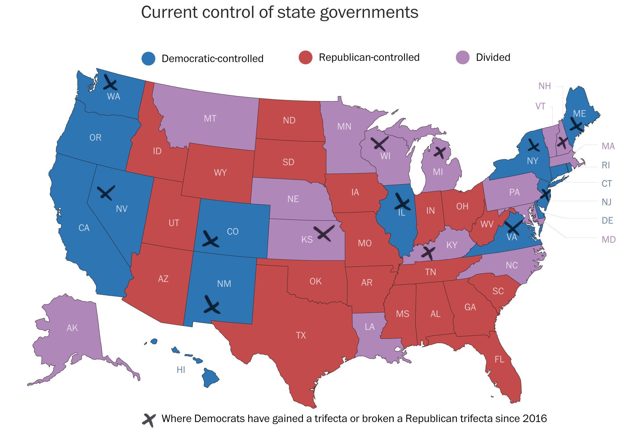
Then we get to a choropleth map. It shows the current state of control for each state.
X marks the spot?However, here the indicator for recent party switches is a set of x’s. These have the same casual approach as the arrows above. But in this case, a careful examination of the x’s indicates they are not unique, like a person drawing a curve with a pen tool. Instead these come from a pre-determined set as the x’s share the exact same shape, stroke lengths and directions.
In years past we probably would have seen the indicator represented by an outline of the state border or a pattern cross-hatching. After all, with the purple being lighter than the blue, the x’s appear more clearly against purple states than blue. I have to admit I did not see New Jersey at first.
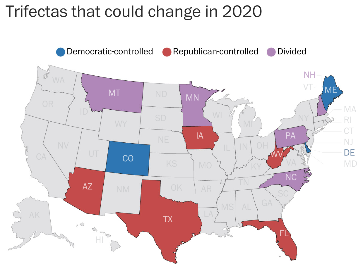
Of course, in an ideal world, a box map would probably be clearer still. But the curious part is that the very next map does a great job of focusing the user’s attention on the datapoint that matters: states set for potential changes next November.
Pennsylvania is among the states…
Here the states of little interest are greyed out. The designers use colour to display the current status of the potential trifecta states. And so I am left curious why the designers did not choose to take a similar approach with the remaining graphics in the piece.
Overall, I should say the piece is strong. The graphics generally work very well. My quibbles are with the aesthetic stylings, which seem out of place for a straight news article. Something like this could work for an opinion piece or for a different subject matter. But for politics it just struck a loud dissonant chord when I first read the piece.
Credit for the piece goes to Kate Rabinowitz and Ashlyn Still.
Last we looked at the revenge of the flyover states, the idea that smaller cities in swing states are trending Republican and defeating the growing Democratic majority in big cities. This week I want to take a look at something a few weeks back, a piece from CityLab about the elections in Virginia, Kentucky, and Mississippi.
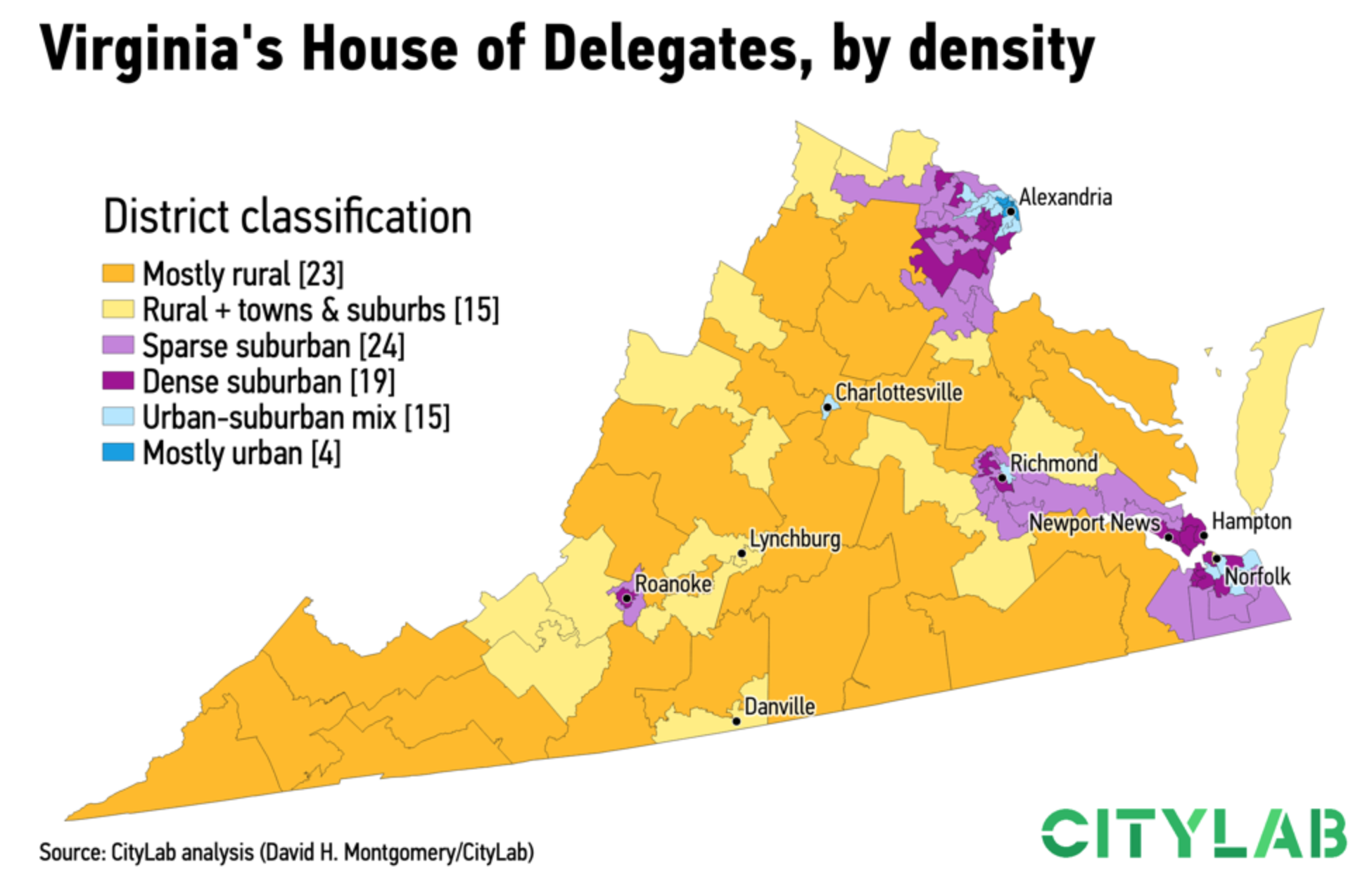
There’s nothing radical in this piece. Instead, it’s some solid uses of line charts and bar charts (though I still don’t generally love them stacked). The big flashy graphic was this, a map of Virginia’s state legislative districts, but mapped not by party but by population density.
Democrats now control a majority of these seats.
It classified districts by how how urban, suburban, or rural (or parts thereof) each district was. Of course the premise of the article is that the suburbs are becoming increasingly Democratic and rural areas increasingly Republican.
But it all goes to show that 2020 is going to be a very polarised year.
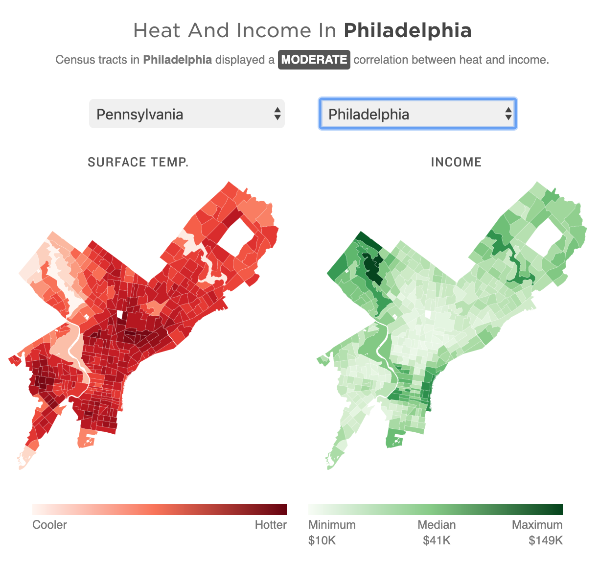
Yesterday was the first day of 32º+C (90º+F) in Philadelphia in October in 78 years. Gross. But it made me remember this piece last month from NPR that looked at the correlation between extreme urban heat islands and areas of urban poverty. In addition to the narrative—well worth the read—the piece makes use of choropleths for various US cities to explore said relationship.
My neighbourhood’s not bad, but thankfully I live next to a park.
As graphics go, these are effective. I don’t love the pure gradient from minimum to maximum, however, my bigger point is about the use of the choropleth compared to perhaps a scatter plot. In these graphics that are trying to show a correlation between impoverished districts and extreme heat, I wonder if a more technical scatterplot showing correlation would be effective.
Another approach could be to map the actual strength of the correlation. What if the designers had created a metric or value to capture the average relationship between income and heat. In that case, each neighbourhood could be mapped as how far above or below that value they are. Because here, the user is forced to mentally transpose the one map atop the other, which is not easy.
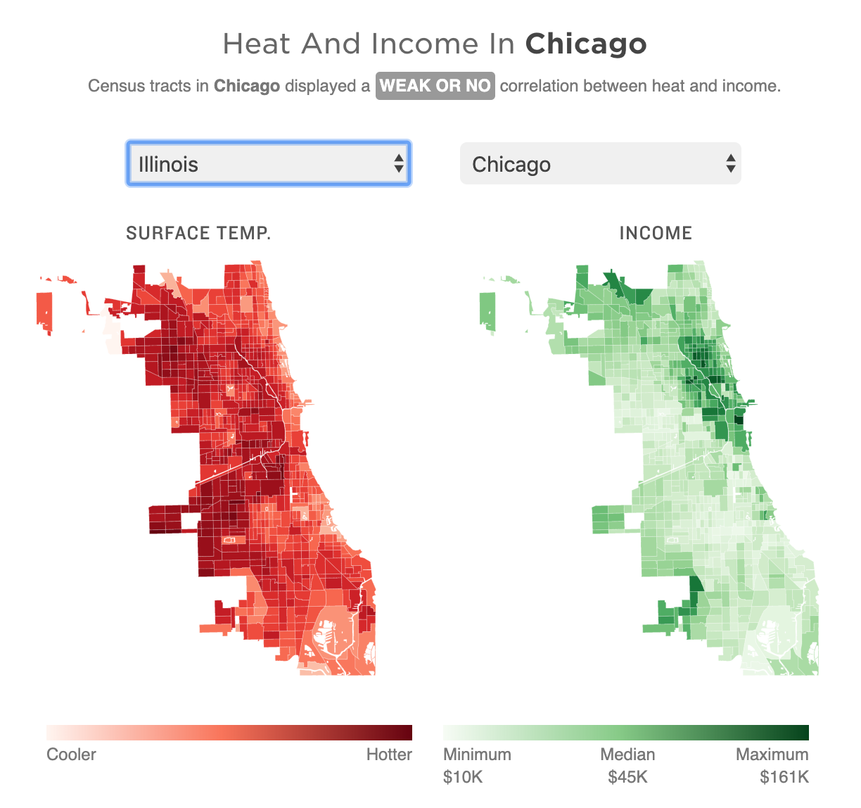
For those of you from Chicago, that city is rated as weak or no correlation to the moderately correlated Philadelphia.
I lived near the lake for eight years, and that does a great deal for mitigating temperature extremes.
Granted, that kind of scatterplot probably requires more explanation, and the user cannot quickly find their local neighbourhood, but the graphics could show the correlation more clearly that way.
Finally, it goes almost without saying that I do not love the red/green colour palette. I would have preferred a more colour-blind friendly red/blue or green/purple. Ultimately though, a clearer top label would obviate the need for any colour differentiation at all. The same colour could be used for each metric since they never directly interact.
Overall this is a strong piece and speaks to an important topic. But the graphics could be a wee bit more effective with just a few tweaks.
Credit for the piece goes to Meg Anderson and Sean McMinn.
Last week was the climate summit in New York, and the science continues to get worse. Any real substantive progress in fighting climate change will require sacrifices and changes to the way our societies function and are organised, including spatially. Because one area that needs to be addressed is the use of personal automobiles that consume oil and emit, among other things, carbon dioxide. But living without cars is not easy in a society largely designed where they are a necessity.
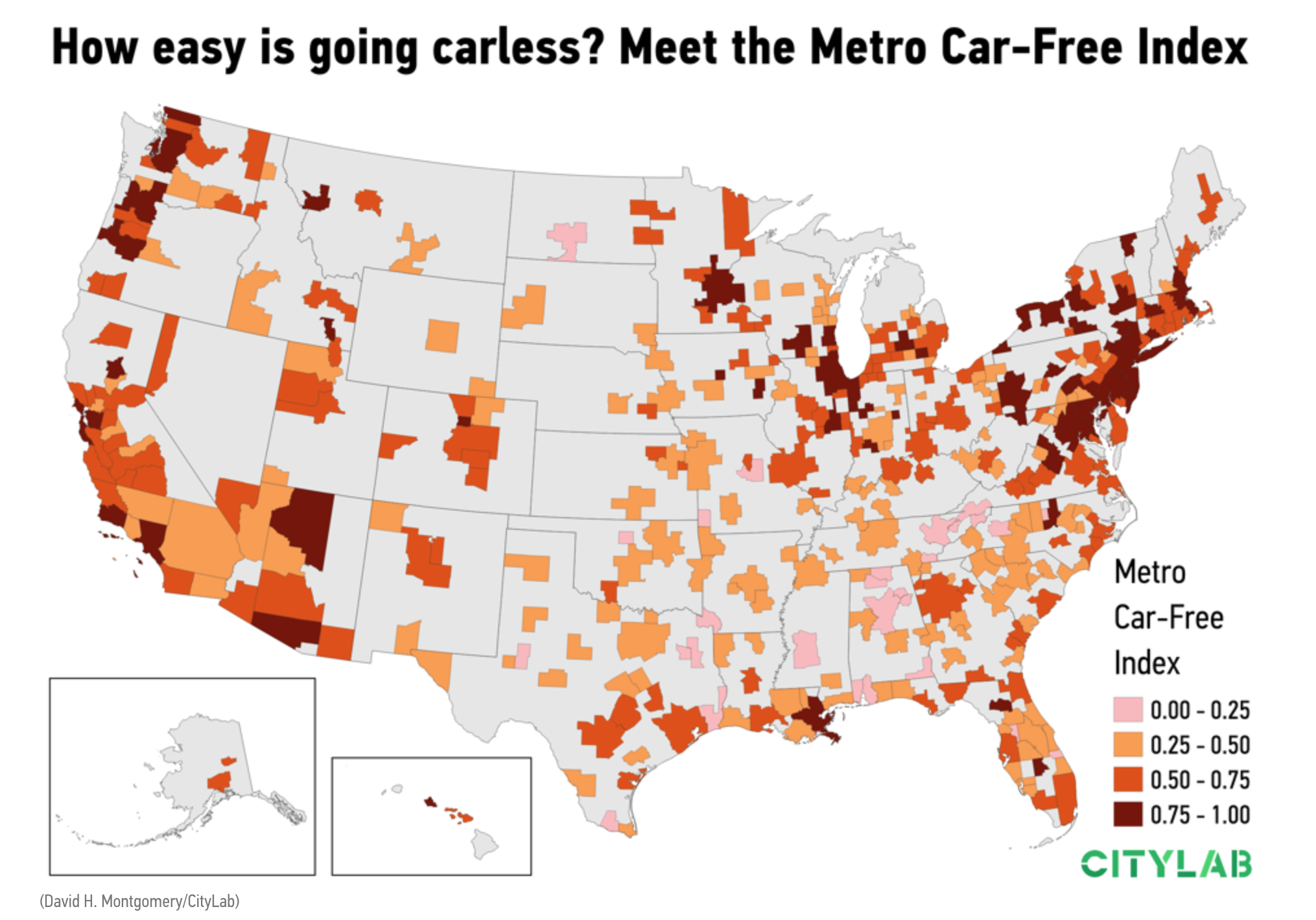
But over at CityLab, Richard Florida and Charlotta Mellander created an index trying to capture the ability to live without a car. The overall piece is worth a read, but as usual I want to focus on the graphic.
The Northeast is where it’s at with its dense cities designed for a pre-automobile era
It’s nothing crazy, but it really does shine as a good example of when to use a map. First, I enjoy seeing metro maps of the United States used as choropleths, which is why I’ve made them as part of job at the Philly Fed. CityLab’s map does a good job showing there is a geographic pattern to the location of cities best situated for those trying to live a car-free life. Perhaps not surprisingly, one of the big clusters is the Northeast Corridor, including Philadelphia, which ranks as the 17th best (out of 398) and the 7th best of large metro areas (defined as more than one million people), beating out Chicago, ranked 23rd and 8th, respectively.
Design wise I have two small issues. First, I might quibble with the colour scheme. I’m not sure there is enough differentiation between the pink and light orange. A very light orange could have perhaps been a better choice. Though I am sympathetic to the need to keep that lowest bin separate from the grey.
Secondly, with the legend, because the index is a construct, I might have included some secondary labelling to help the reader understand what the numbers mean. Perhaps an arrow and some text saying something like “Easier car-free living”. Once you have read the text, it makes sense. However, viewing the graphic in isolation might not be as clear as it could be with that labelling.
So admittedly this post should have been up last week, but I liked the lunar cycle one too much. But today is Friday and who cares. We made it to the end of the week.
In the wake of the shootings last week, someone on Twitter posed the question:
Legit question for rural Americans – How do I kill the 30-50 feral hogs that run into my yard within 3-5 mins while my small kids play?
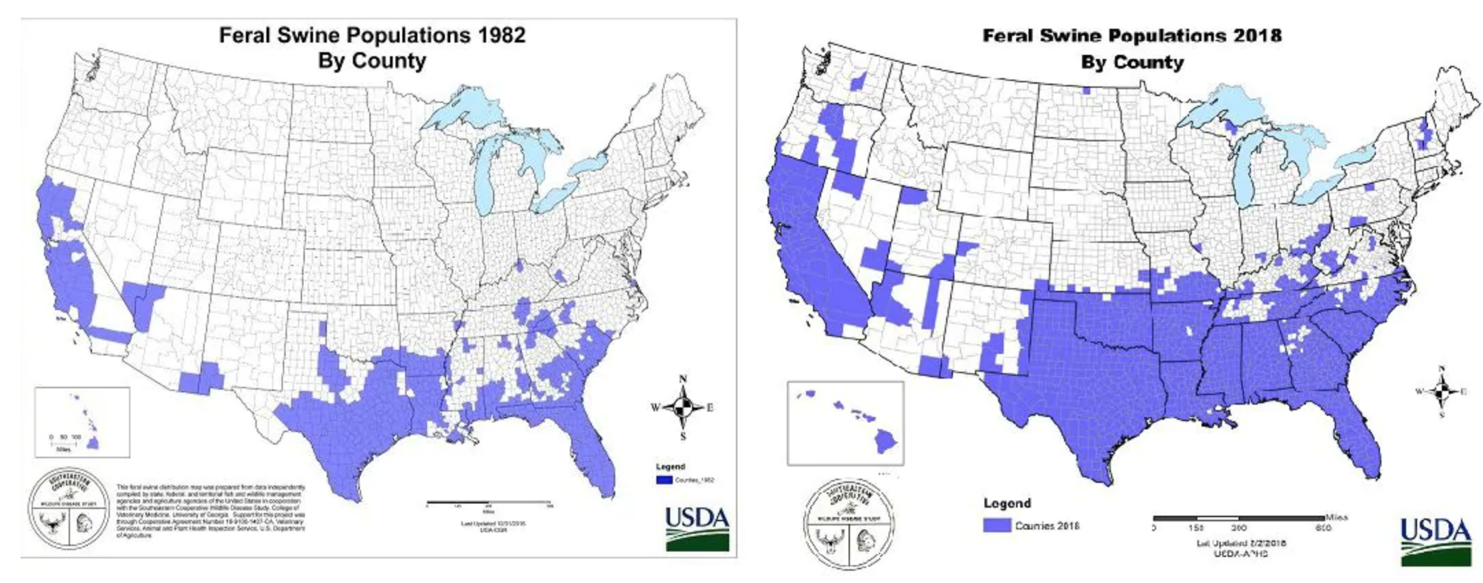
And with that the Internet was off. Memes exploded across the social media verse. Thankfully the Washington Post took it seriously and found data on the expanding footprint of hogs in the United States.
Pig problems
The article also points out, however, that the firearm that prompted the discussion, the now infamous AR-15, would also be a poor choice against feral hogs as its too small a calibre to effectively deal with the animals.
Credit for the piece goes to the US Department of Agriculture.
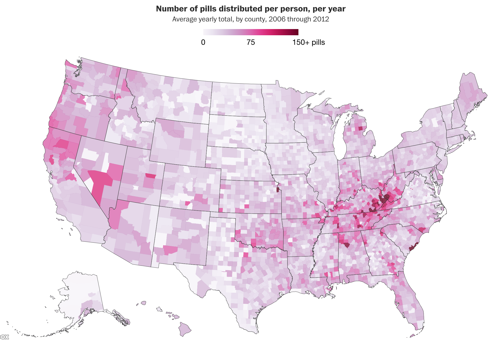
Two weeks ago the Washington Post published a fascinating article detailing the prescription painkiller market in the United States. The Drug Enforcement Administration made the database available to the public and the Post created graphics to explore the top-line data. But the Post then went further and provided a tool allowing users to explore the data for their own home counties.
The top line data visualisation is what you would expect: choropleth maps showing the prescription and death rates. This article is a great example of when maps tell stories. Here you can clearly see that the heaviest hit areas of the crisis were Appalachia. Though that is not to say other states were not ravaged by the crisis.
There are some clear geographic patterns to see here
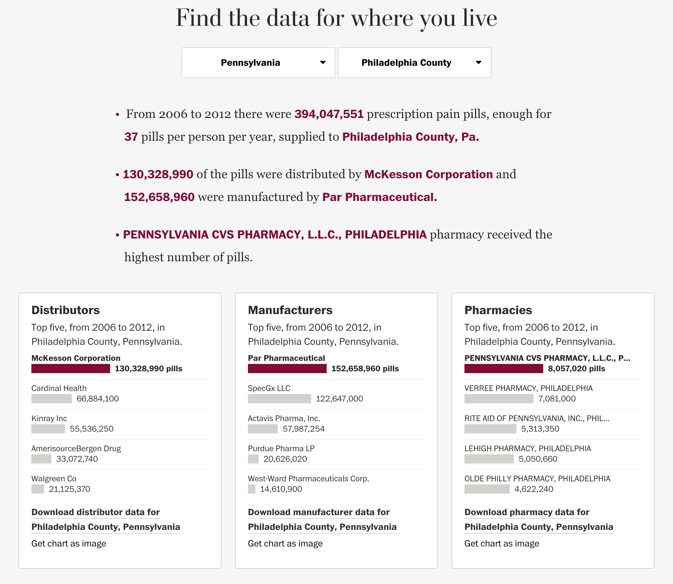
For me, however, the true gem in this piece is the tool allowing you the user to find information on your county. Because the data is granular down to county-level information on things like pill shipments from manufacturer to distributor, we can see which pharmacies were receiving the most pills. And, crucially, which manufacturers were flooding the markets. For this screenshot I looked at Philadelphia, though I only moved here in 2016, well after the date range for this data set.
It could be worse
You can clearly see, however, the designers chose simple bar charts to show the top-five. I don’t know if the exact numbers are helpful next to the bars. Visually, it becomes a quick mess of greys, blacks, and burgundies. A quieter approach may have allowed the bars to really shine while leaving the numbers, seemingly down to the tens, for tables. I also cannot figure out why, typographically, the pharmacies are listed in all capitals.
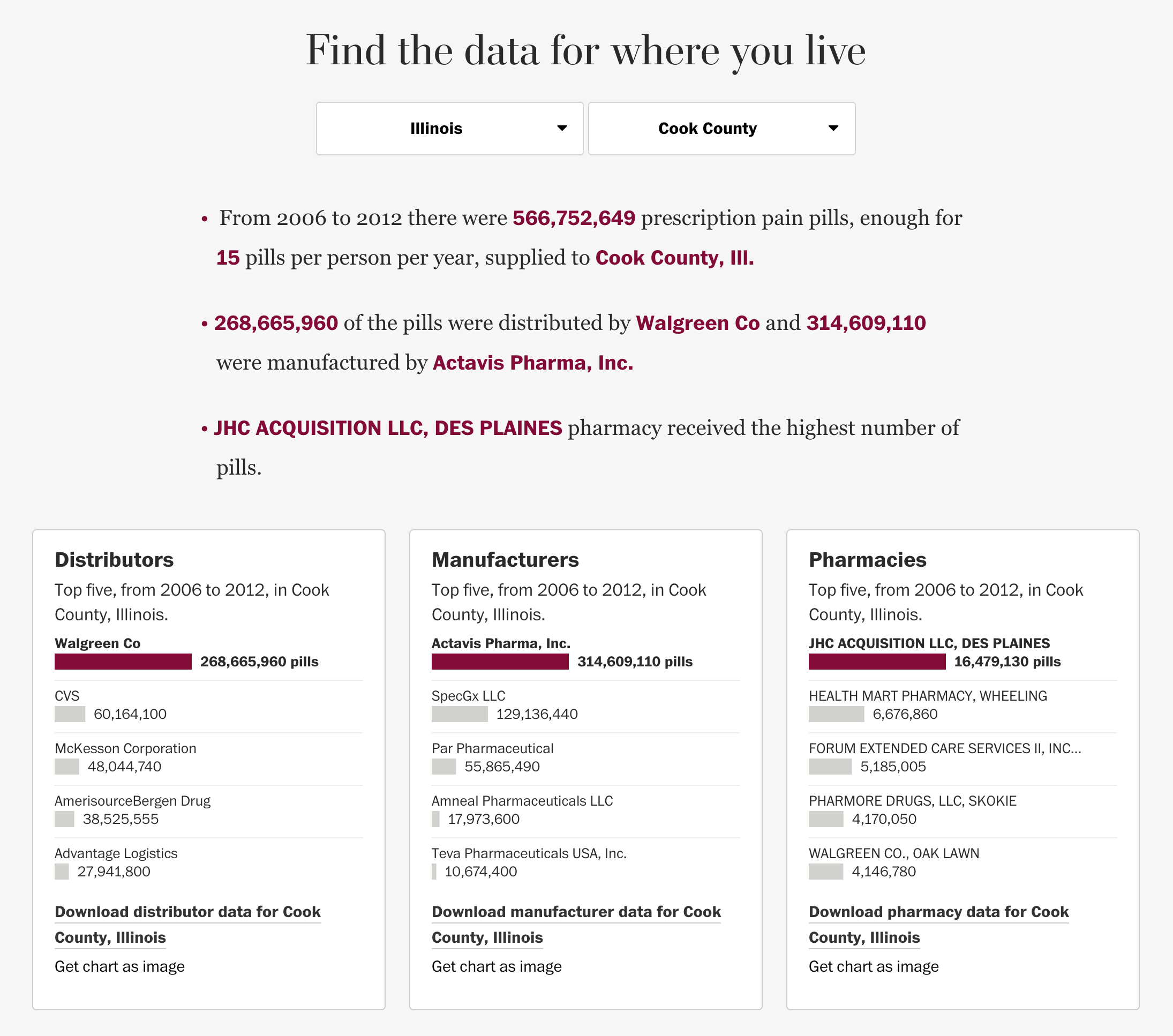
But the because I lived in Chicago for most of the crisis, here is the screenshot for Cook County. Of course, for those not from Chicago, it should be pointed out that Chicago is only a portion of Cook County, there are other small towns there. And some of Chicago is within DuPage County. But, still, this is pretty close.
Better numbers than Philly
In an unrelated note, the bar charts here do a nice job of showing the market concentration or market power of particular companies. Compare the dominance of Walgreens as a distributor in Cook County compared to McKesson in Philadelphia. Though that same chart also shows how corporate structures can obscure information. I was never far from a big Walgreens sign in Chicago, but I have never seen a McKesson Corporation logo flying outside a pharmacy here in Philadelphia.
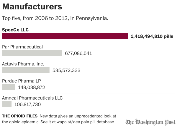
Lastly, the neat thing about this tool is that the user can opt to download an image of the top-five chart. I am not sure how useful that bit is. But as a designer, I do like having that functionality available. This is for Pennsylvania as a whole.
For Pennsylvania, state-wide
Credit for the piece goes to Armand Emamdjomeh, Kevin Schaul, Jake Crump and Chris Alcantara.