Yesterday we looked at the New York Times coverage of some water stress climate data and how some US cities fit within the context of the world’s largest cities. Well today we look at how the Washington Post covered the same data set. This time, however, they took a more domestic-centred approach and focused on the US, but at the state level.
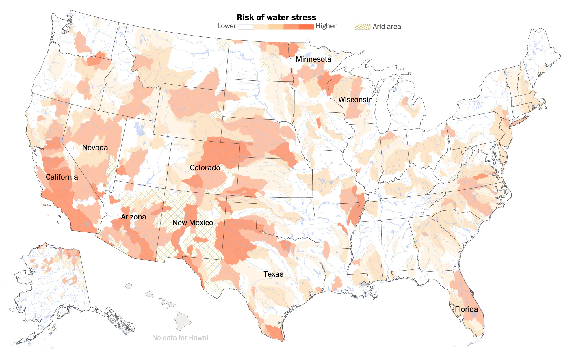
Both pieces start with a map to anchor the piece. However, whereas the Times began with a world map, the Post uses a map of the United States. And instead of highlighting particular cities, it labels states mentioned in the following article.
Interestingly, whereas the Times piece showed areas of No Data, including sections of the desert southwest, here the Post appears to be labelling those areas as “arid area”. We also see two different approaches to handling the data display and the bin ranges. Whereas the Times used a continuous gradient the Post opts for a discrete gradient, with sharply defined edges from one bin to the next. Of course, a close examination of the Times map shows how they used a continuous gradient in the legend, but a discrete application. The discrete application makes it far easier to compare areas directly. Gradients are, by definition, harder to distinguish between relatively close areas.
The next biggest distinguishing characteristic is that the Post’s approach is not interactive. Instead, we have only static graphics. But more importantly, the Post opts for a state-level approach. The second graphic looks at the water stress level, but then plots it against daily per capita water use.
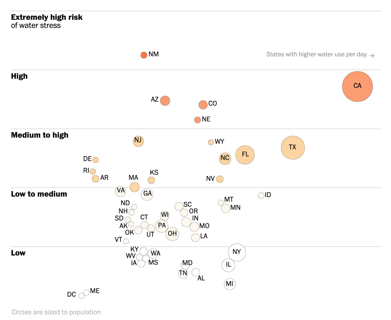
My question is from the data side. Whence does the water use data come? It is not exactly specified. Nor does the graphic provide any axis limits for either the x- or the y-axis. What this graphic did make me curious about, however, was the cause of the high water consumption. How much consumption is due to water-intensive agricultural purposes? That might be a better use of the colour dimension of the graphic than tying it to the water stress levels.
The third graphic looks at the international dimension of the dataset, which is where the Times started.
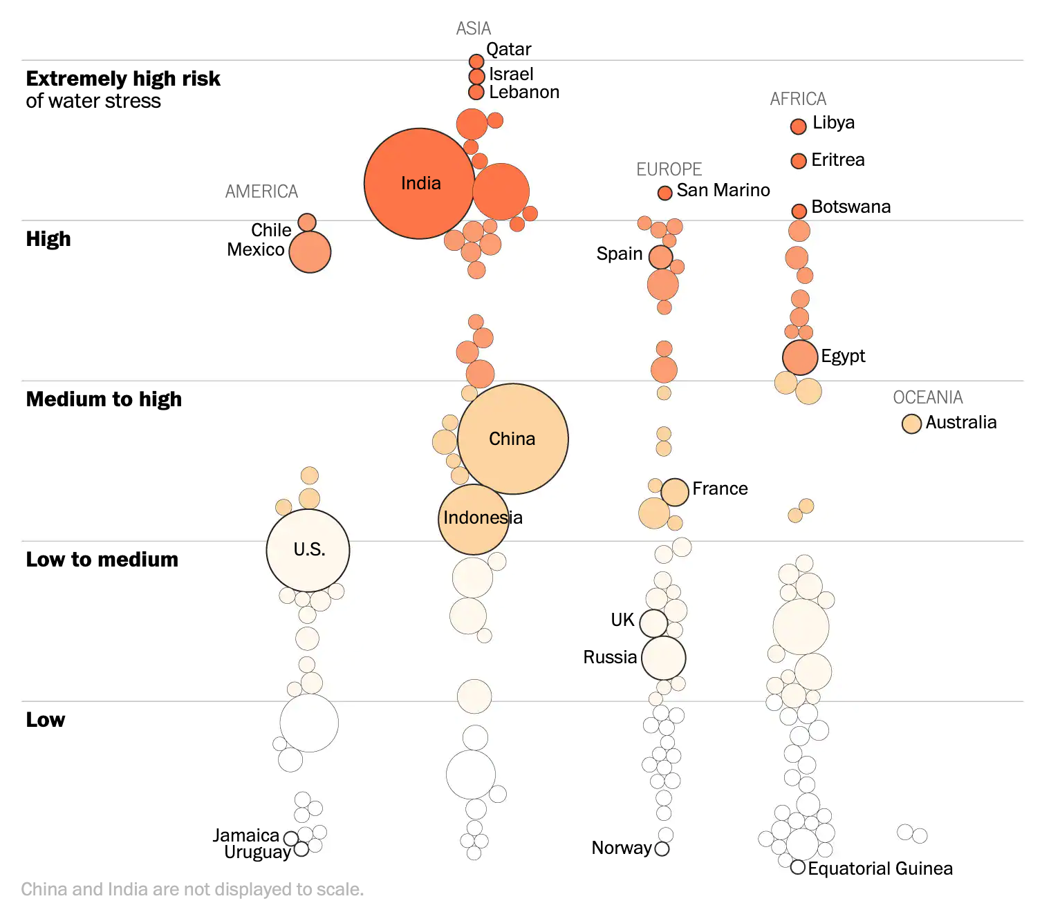
Here we have an interesting use of area to size population. In the second graphic, each state is sized by population. Here, we have countries sized by population as well. Except, the note at the bottom of the graphic notes that neither China nor India are sized to scale. And that make sense since both countries have over a billion people. But, if the graphic is trying to use size in the one dimension, it should be consistent and make China and India enormous. If anything, it would show the scale of the problem of being high stress countries with enormous populations.
I also like how in this graphic, while it is static in nature, breaks each country into a regional classification based upon the continent where the country is located.
Overall this, like the Times piece, is a solid graphic with a few little flaws. But the fascinating bit is how the same dataset can create two stories with two different foci. One with an international flavour like that of the Times, and one of a domestic flavour like this of the Post.
Credit for the piece goes to Bonnie Berkowitz and Adrian Blanco.
Leave a Reply
You must be logged in to post a comment.